Detecting Pneumonia in Chest X-Ray Images Using Deep Learning Models on Google Colab Pro

บทความโดย ผศ.ดร.ณัฐโชติ พรหมฤทธิ์
ภาควิชาคอมพิวเตอร์
คณะวิทยาศาสตร์
มหาวิทยาลัยศิลปากร
บทความนี้เราจะพัฒนา Deep Learning Model แบบ Binary Classification และ Multi-Class Classification เพื่อตรวจจับโรคปอดอักเสบ (นิวโมเนีย - Pneumonia) หรือโรคปอดบวม ด้วยภาพ X-Ray ปอด ซึ่งจะมีการโหลด Image Dataset มาจาก Folder บน Google Colab ที่นำมาจาก kaggle.com อีกที
นอกจากจะได้เห็นการพัฒนา Model สองแบบ สำหรับตรวจจับโรคปอดอักเสบแล้ว ผู้อ่านจะได้เห็นตัวอย่างการทำ Augmentation ซึ่งเป็นเทคนิคการขยายขนาด Dataset และเพิ่มความหลากหลายของภาพเพื่อลด Generalization Error ของ Model อีกด้วย
Pneumonia X-Ray Images Dataset
Pneumonia X-Ray Images เป็น Dataset ที่มี 2 Class คือ ภาพ X-Ray ปอดปกติ (Normal) และภาพ X-Ray ปอดอักเสบ (Opacity หรือ Pneumonia) รวมทั้งหมด 5,856 ภาพ ซึ่งแบ่งเป็น
Training Dataset 4,192 ภาพ (Normal Cases 1,082 ภาพ และ Lung Opacity Cases 3,110 ภาพ)
Validation Dataset 1,040 ภาพ (Normal Cases 267 ภาพ และ Lung Opacity Cases 773 ภาพ)
Testing Dataset 624 ภาพ (Normal Cases 234 ภาพ และ Lung Opacity Cases 390 ภาพ)
โดยเราจะนำมันมาจาก kaggle.com ผ่านทาง Kaggle API ตามขั้นตอน ดังต่อไปนี้
- Login ที่ www.kaggle.com คลิ๊กที่ Profile Image แล้วคลิ๊ก Account

- Download ไฟล์ kaggle.json โดยคลิ๊กที่ Create New API Token

- ไปที่ Google Colab แล้วคลิ๊ก NEW NOTEBOOK ตั้งชื่อไฟล์ แล้วเลือกเมนู Runtime -> Change runtime type
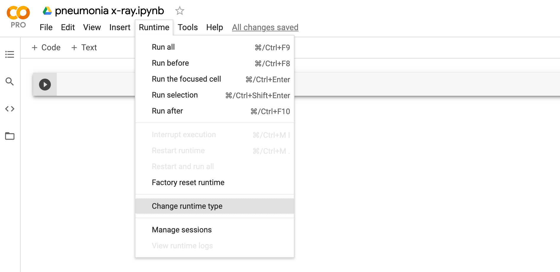
- เลือกชนิดของ Hardware accelerator เป็น GPU และ Runtime shape เป็น High-RAM (ถ้าใช้ Google Colab Pro) แล้วคลิ๊ก SAVE

- ตรวจสอบการใช้งาน GPU ด้วยคำสั่งต่อไปนี้
!nvidia-smi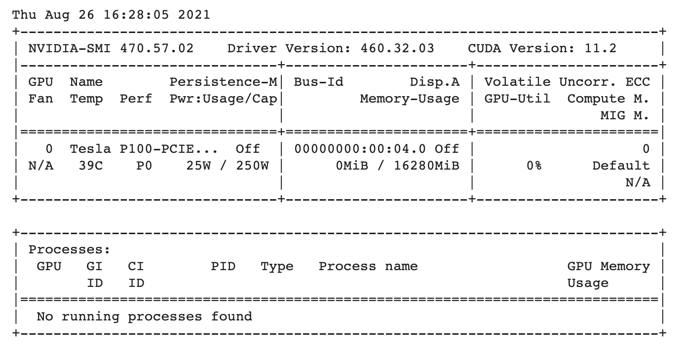
- ติดตั้ง Kaggle Library
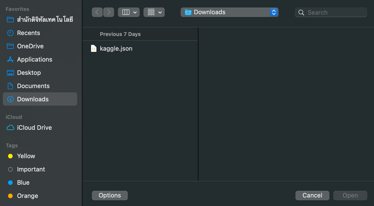
!pip install kaggle- รัน Code ต่อไปนี้แล้ว Upload kaggle.json โดยการคลิ๊กที่ Choose Files เลือกไฟล์ kaggle.json ใน Folder Download แล้วคลิ๊กปุ่ม Open
from google.colab import files

files.upload()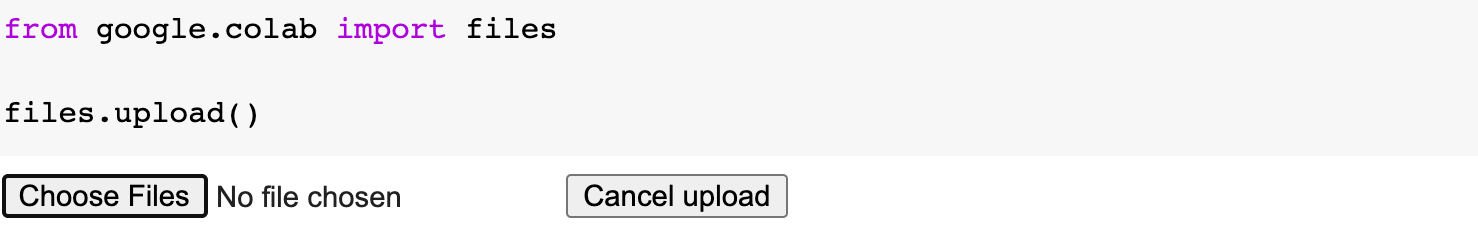
- สร้าง Folder kaggle บน Google Colab เพื่อเก็บไฟล์ kaggle.json
!mkdir kaggle- ย้ายไฟล์ kaggle.json ไปยัง Folder kaggle
!mv kaggle.json kaggle- เปลี่ยน Permission ของไฟล์ kaggle.json
!chmod 600 /content/kaggle/kaggle.json- Config Kaggle Environment
import os

os.environ['KAGGLE_CONFIG_DIR'] = "/content/kaggle"- ไปที่ Pneumonia X-Ray Images คลิ๊กที่ icon 3 จุด (แนวตั้ง) แล้วเลือก Copy API command
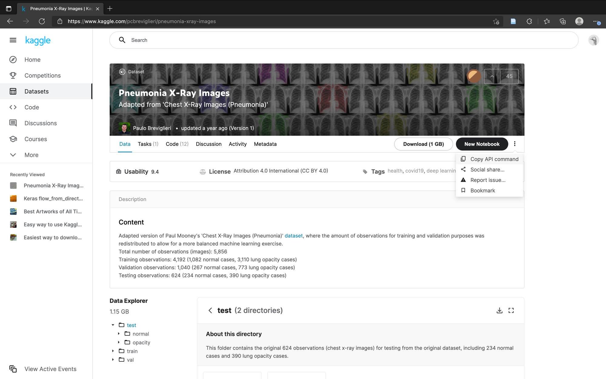
- นำคำสั่งที่ Copy มารันบน Colab Notebook (โดยเติม ! หน้าคำสั่ง) เพื่อ Download Pneumonia X-Ray Images Dataset
!kaggle datasets download -d pcbreviglieri/pneumonia-xray-images
- สร้าง Folder pneumonia-xray-images แล้ว Unzip Dataset
!mkdir pneumonia-xray-images && unzip -q pneumonia-xray-images.zip -d pneumonia-xray-imagesซึ่งภายใน pneumonia-xray-images จะมี Folder ต่างๆ ที่เก็บภาพ X-ray ปอด สำหรับการ Train, Validate และ Test ดังต่อไปนี้
.
├── test
│   ├── normal
│   └── opacity
├── train
│   ├── normal
│   └── opacity
└── val
    ├── normal
└── opacity- Import Library และกำหนดค่า Parameter ที่จำเป็น
import tensorflow as tf
to_categorical = tf.keras.utils.to_categorical

array_to_img = tf.keras.preprocessing.image.array_to_img
ReduceLROnPlateau = tf.keras.callbacks.ReduceLROnPlateau
ImageDataGenerator = tf.keras.preprocessing.image.ImageDataGenerator

from sklearn.metrics import classification_report
from sklearn.metrics import roc_curve, auc

import matplotlib.pyplot as plt

import plotly
import plotly.graph_objs as go
import plotly.figure_factory as ff
import plotly.express as px

import numpy as np
from collections import Counter
from sklearn.utils.class_weight import compute_class_weight
from sklearn.metrics import confusion_matrix

import pandas as pd
img_rows, img_cols = 350, 350
batch_size = 32
epochs = 15
num_classes = 2
seed = 1

input_shape = (img_rows, img_cols, 1)
เนื่องจากภาพต้นฉบับทั้งหมดใน Dataset มีความสูงและความยาวมากกว่า 1,000 Pixel เราจึงต้องลดขนาดลงให้สามารถนำเข้ามา Train ใน Model ได้โดยใช้เวลาในการ Train แต่ละ Epoch ไม่มากนัก แต่ยังคงมีประสิทธิภาพที่ดี นอกจากนี้การปรับ Batch Size ก็มีผลต่อประสิทธิภาพของ Model เช่นกัน เพื่อจะให้ได้ผลลัพธ์ที่ดีที่สุด ในการทดลองจึงควรมีการปรับขนาด Batch Size ด้วยครับ
Binary Classification Model
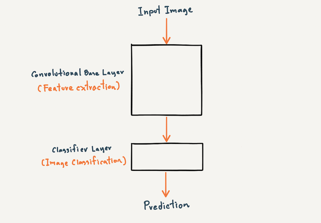
เพื่อจะทำนายว่าปอดอักเสบหรือไม่ เราสามารถพัฒนา Model ได้ทั้งแบบ Binary Classification และ Multi-Class Classification ซึ่งทั้ง 2 Model เราจะใช้ CNN Layer รับภาพขนาด 350x350 Pixel เพื่อทำ Feature Extraction และใช้ Dense Layer ในการทำ Image Classification ดังภาพ
สำหรับการนิยาม Model แบบ Binary Classification และ Multi-Class Classification จะมีการกำหนดจำนวน Output Node และ Activate Function ที่ Output Layer รวมทั้ง Loss Function ที่แตกต่างกัน ดังนี้
Binary Classification Model กำหนด Activate Function แบบ Sigmoid กำหนด Loss Function แบบ Binary Crossentropy และกำหนด Output Node = 1
Multi-Class Classification Model กำหนด Activate Function แบบ Softmax กำหนด Loss Function แบบ Categorical Crossentropy และ Output Node = 2
Load Dataset From Directory
เราจะ Load ภาพ จาก Folder pneumonia-xray-images โดยใช้ ImageDataGenerator ของ Tensorflow Library ตามขั้นตอนดังนี้
- สร้าง ImageDataGenerator 2 ตัวแปร ได้แก่ datagen และ val_test_datagen
datagen สำหรับอ่านไฟล์ภาพ แล้วทำ Scaling และทำ Image Augmentation เพื่อขยายขนาด Dataset และเพิ่มความหลากหลายของภาพ ด้วยการบิดภาพ (Shear) แบบสุ่มไม่เกิน 20 องศา ขยายภาพ (Zoom) แบบสุ่มไม่เกิน 20% และพลิกภาพแนวนอน (Horizontal Flip) ซ้าย-ขวาแบบสุ่ม
val_test_datagen สำหรับอ่านไฟล์ภาพ แล้วทำ Scaling โดยไม่มีการทำ Image Augmentation เนื่องจากเป็นชุดภาพสำหรับการ Validate และ Test
datagen = ImageDataGenerator(rescale = 1./255,
                             shear_range = 0.2,
                             zoom_range = 0.2,
                             horizontal_flip = True)

val_test_datagen = ImageDataGenerator(rescale = 1./255)- Load ภาพสำหรับการ Train แบบ Grayscale ด้วย datagen จาก Folder pneumonia-xray-images/train/ โดยมีการ Resize ภาพตามความสูงและความกว้างที่กำหนด (350x350) รวมทั้งกำหนด class_mode เป็น Binary เพื่อกำหนด Format ของผลเฉลย และสุ่มภาพเพื่อนำมา Plot ให้เราเห็น
train_it = datagen.flow_from_directory('pneumonia-xray-images/train/',
                                       target_size=(img_rows, img_cols),
                                       batch_size=batch_size,
                                       class_mode='binary',
                                       shuffle=True,
                                       color_mode='grayscale',
                                       seed=seed)
Found 4192 images belonging to 2 classes.
- Load ภาพสำหรับการ Validate และ Test แบบ Grayscale ด้วย val_test_datagen จาก Folder pneumonia-xray-images/val/ และ pneumonia-xray-images/test/ โดยมีการ Resize ภาพตามความสูงและความกว้างที่กำหนดไว้ รวมทั้งกำหนด class_mode เป็น Binary เพื่อกำหนด Format ของผลเฉลย
val_it = val_test_datagen.flow_from_directory('pneumonia-xray-images/val/',
                                              target_size=(img_rows, img_cols),
                                              batch_size=batch_size,
                                              class_mode='binary',
                                              shuffle=False,
                                              color_mode='grayscale')
test_it = val_test_datagen.flow_from_directory('pneumonia-xray-images/test/',
                                               target_size=(img_rows, img_cols),
                                               batch_size=batch_size,
                                               class_mode='binary',
                                               shuffle=False,
                                               color_mode='grayscale')
Found 1040 images belonging to 2 classes.
Found 624 images belonging to 2 classes.
- สรุปข้อมูลของแต่ละ Batch
batchX, batchY = next(train_it)
print('Batch shape=%s, min=%.3f, max=%.3f' % (batchX.shape, batchX.min(), batchX.max()))
Batch shape=(32, 350, 350, 1), min=0.000, max=1.000
- ดึงชื่อ Class ที่ได้จากชื่อ Folder ย่อย ใน Folder pneumonia-xray-images/train/ มาเก็บที่ตัวแปร labels
labels = list(train_it.class_indices.keys())
labels
['normal', 'opacity']
- นับจำนวนภาพของ Class ต่างๆ จาก Train Dataset
Counter(train_it.classes)Counter({0: 1082, 1: 3110})
ซึ่งพบว่าจำนวนภาพจาก 2 Class ของ Train Dataset มีลักษณะแบบ Imbalanced คือ ทั้ง 2 Class มีจำนวนไม่เท่ากัน ดังนั้นเราจะคำนวณค่า Weight ของแต่ละ Class (Class Weight) เพื่อเป็น Parameter ในรูปแบบของ Dict (Key กับ Value) ตอน Train Model ครับ
- คำนวณค่า Class Weight โดยการให้น้ำหนัก Class ที่มีจำนวนภาพน้อย มากกว่า Class ที่มีจำนวนภาพมากกว่า
weights = compute_class_weight(class_weight = 'balanced', classes = np.unique(train_it.classes), y = train_it.classes)
weights
array([1.93715342, 0.67395498])
cw = dict(zip(np.unique(train_it.classes), weights))
cw
{0: 1.9371534195933457, 1: 0.6739549839228296}
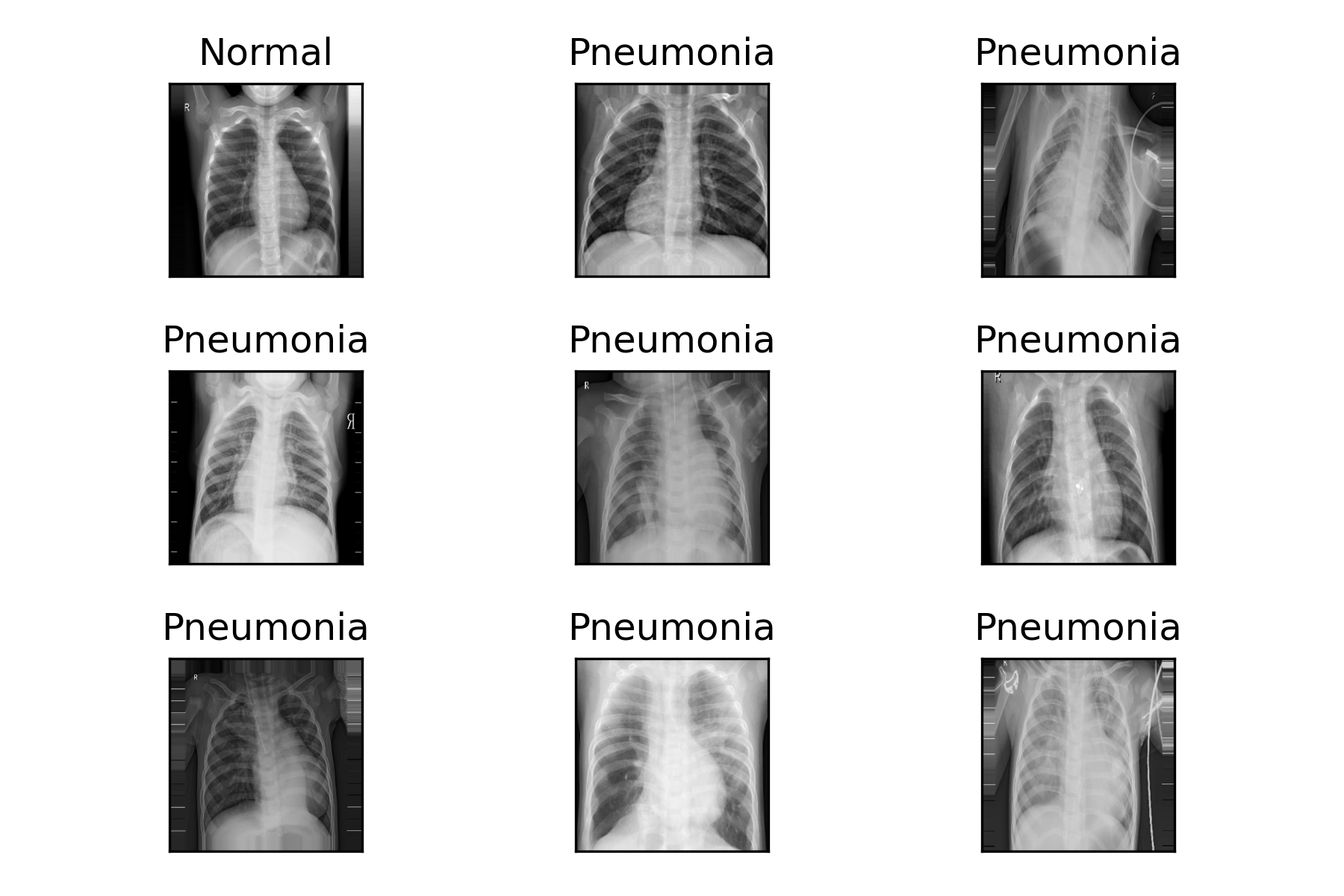
- แสดงภาพตัวอย่างจาก Train Dataset
for i in range(9):
    ax = plt.subplot(3, 3, 1+i)
    ax.set_xticks([])
    ax.set_yticks([])
    ax.set_title('%s'%(labels[int(batchY[i])]))
    plt.imshow(batchX[i][:,:,0], cmap=plt.get_cmap('gray'))

plt.tight_layout()
plt.savefig('chest_xray.png', dpi=300)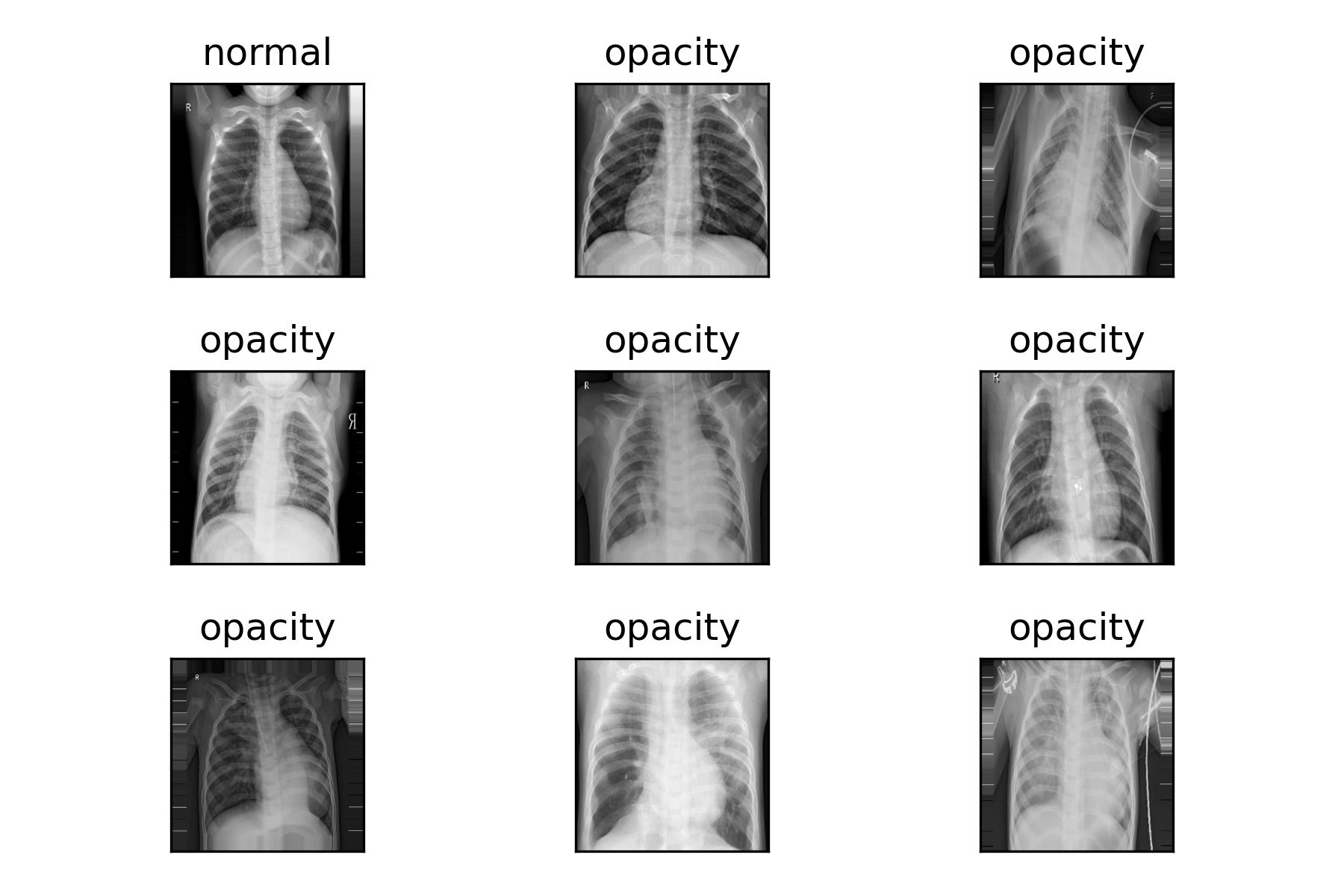
Train Model
- นิยาม Model แบบ Convolutional Neural Network (CNN) โดยกำหนด Activate Function แบบ Sigmoid และกำหนด Output Node = 1 ใน Layer สุดท้าย
#Feature Extraction
model = tf.keras.Sequential()
model.add(tf.keras.layers.Input(shape=input_shape))
model.add(tf.keras.layers.Conv2D(32, kernel_size=(3, 3), activation='relu', input_shape=input_shape))
model.add(tf.keras.layers.MaxPooling2D(pool_size=(2, 2)))

model.add(tf.keras.layers.Conv2D(32, kernel_size=(3, 3), activation='relu'))
model.add(tf.keras.layers.MaxPooling2D(pool_size=(2, 2)))

model.add(tf.keras.layers.Conv2D(64, kernel_size=(3, 3), activation='relu'))
model.add(tf.keras.layers.MaxPooling2D(pool_size=(2, 2)))

model.add(tf.keras.layers.Conv2D(64, kernel_size=(3, 3), activation='relu'))
model.add(tf.keras.layers.MaxPooling2D(pool_size=(2, 2)))

#Image Classification
model.add(tf.keras.layers.Flatten())
model.add(tf.keras.layers.Dense(128, activation='relu'))
model.add(tf.keras.layers.Dense(64, activation='relu'))
model.add(tf.keras.layers.Dense(1, activation='sigmoid'))- Compile Model โดยกำหนด Loss Function แบบ Binary Crossentropy
model.compile(loss='binary_crossentropy', optimizer='adam', metrics=['accuracy'])
model.summary()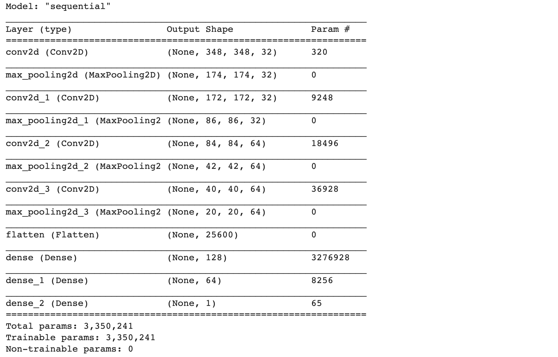
- คำนวณ Step ของการ Train การ Validate และการ Test
STEP_SIZE_TRAIN=train_it.n//train_it.batch_size
STEP_SIZE_VALID=val_it.n//val_it.batch_size
STEP_SIZE_TEST=test_it.n//test_it.batch_size- กำหนด Callbacks เพื่อปรับลด Learning Rate ด้วยการคูณกับค่า Factor เมื่อค่า val_loss เพิ่มขึ้นมากกว่าค่า val_loss น้อยที่สุด (Plateau) ในขณะที่ Train Model
learning_rate_reduction = ReduceLROnPlateau(monitor='val_loss', patience = 2, verbose=1,factor=0.1, min_lr=0.000001)
callbacks_list = [learning_rate_reduction]- Train Model โดยกำหนดให้ class_weight เท่ากับ cw และสุ่มภาพสำหรับ Train และ Validate
his = model.fit(
        train_it,
        validation_data=val_it,
        epochs=epochs,
        class_weight=cw,
        callbacks=callbacks_list,
        shuffle=True,
        steps_per_epoch=STEP_SIZE_TRAIN,
        validation_steps=STEP_SIZE_VALID)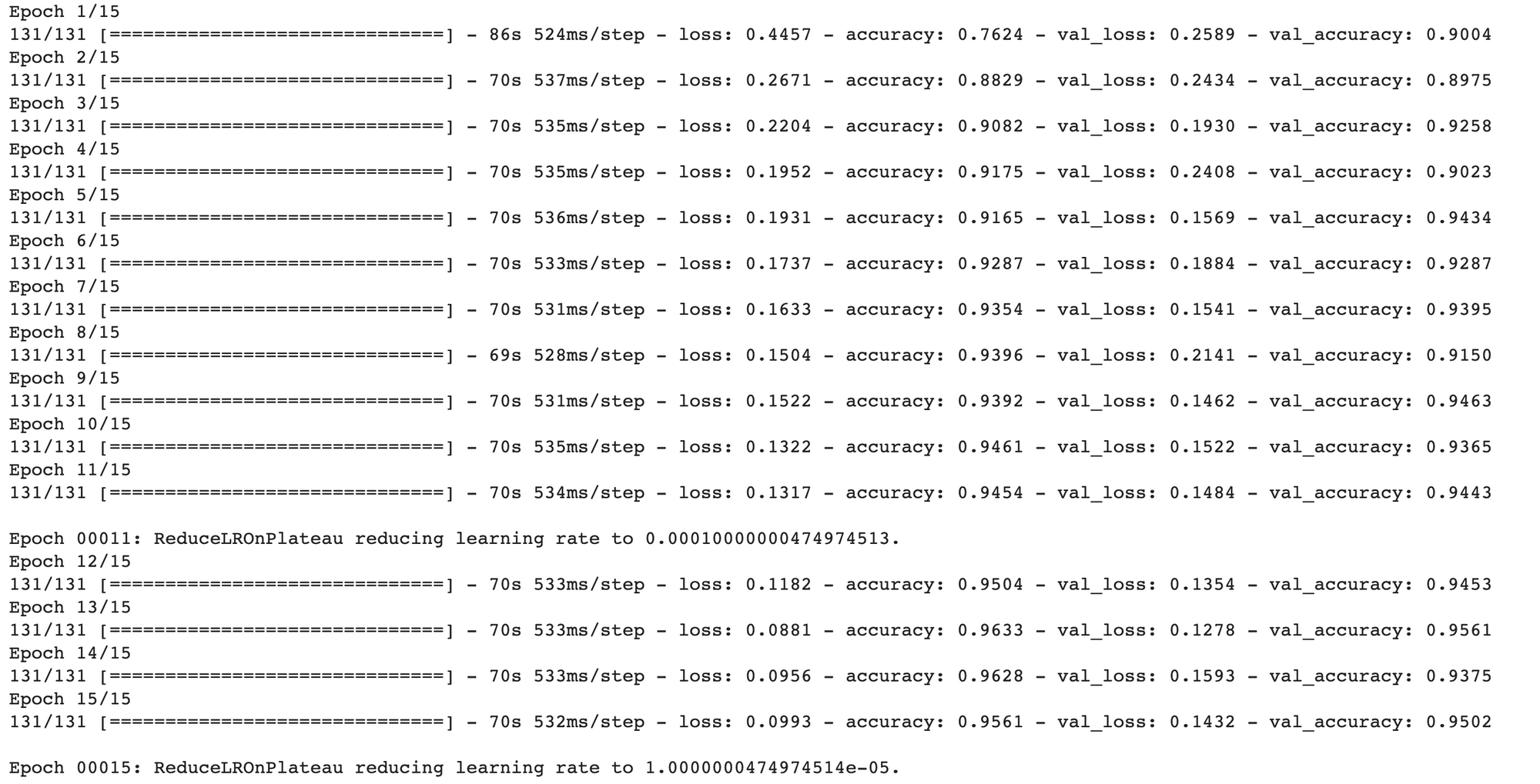
- Plot Loss
h1 = go.Scatter(y=his.history['loss'],
                    mode="lines",
                    line=dict(
                        width=2,
                        color='blue'),
                        name="loss"
                   )
h2 = go.Scatter(y=his.history['val_loss'],
                    mode="lines",
                    line=dict(
                        width=2,
                        color='red'),
                        name="val_loss"
                   )

data = [h1,h2]
layout1 = go.Layout(title='Loss',
                   xaxis=dict(title='epochs'),
                   yaxis=dict(title=''))
fig1 = go.Figure(data, layout=layout1)
plotly.offline.iplot(fig1)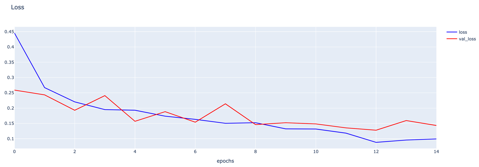
- Plot Accuracy
h1 = go.Scatter(y=his.history['accuracy'],
                    mode="lines", line=dict(
                    width=2,
                    color='blue'),
                    name="acc"
                   )
h2 = go.Scatter(y=his.history['val_accuracy'],
                    mode="lines", line=dict(
                    width=2,
                    color='red'),
                    name="val_acc"
                   )

data = [h1,h2]
layout1 = go.Layout(title='Accuracy',
                   xaxis=dict(title='epochs'),
                   yaxis=dict(title=''))
fig1 = go.Figure(data = data, layout=layout1)
plotly.offline.iplot(fig1)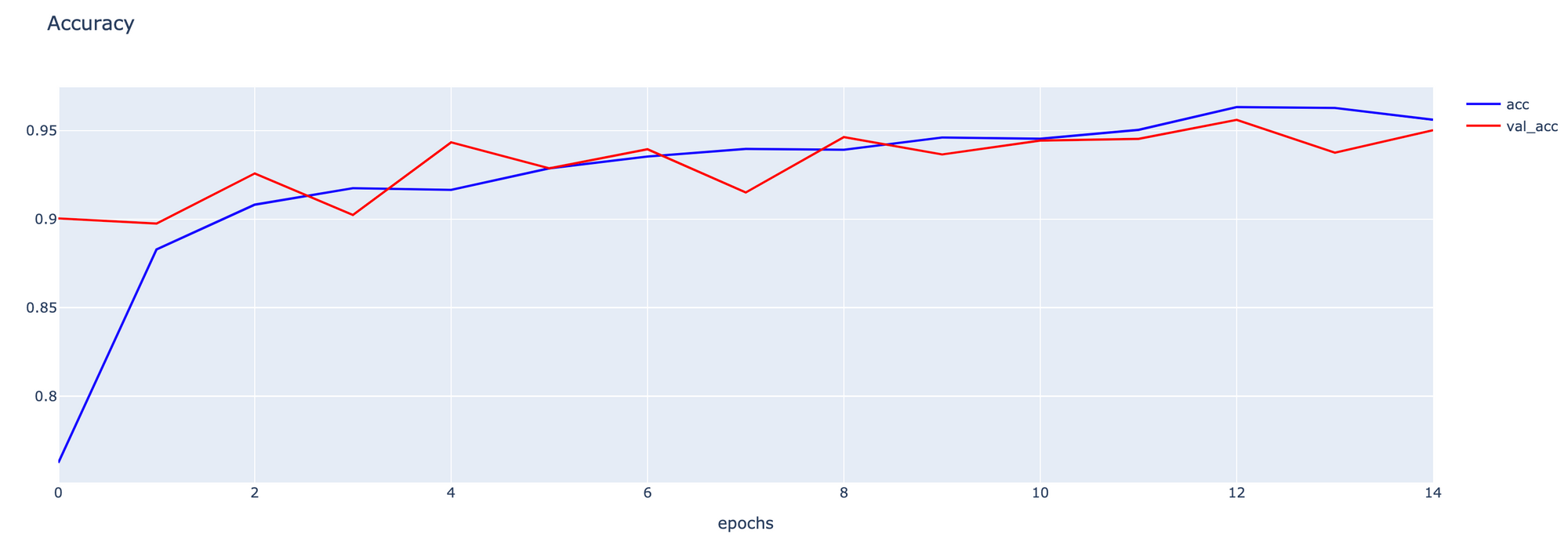
Binary Classification Evaluation
- Predict โรคปอดอักเสบด้วย Test Dataset โดยกำหนดค่า Threshold = 0.5
predicted_classes = (model.predict(test_it, verbose=1) > 0.5).astype("int32")[:,0]20/20 [==============================] - 5s 218ms/step
- แสดงตัวอย่างผลการ Predict และผลเฉลยของ Test Dataset
predicted_classes[:10]array([0, 0, 0, 0, 0, 0, 0, 0, 0, 0], dtype=int32)
test_it.classes[:10]array([0, 0, 0, 0, 0, 0, 0, 0, 0, 0], dtype=int32)
- นิยาม cm_plot Function
def cm_plot(cm, labels):
    x = labels
    y = labels

    z_text = [[str(y) for y in x] for x in cm]
    fig = ff.create_annotated_heatmap(cm, x=x, y=y, annotation_text=z_text, colorscale='blues')

    fig.update_layout(title_text='Confusion Matrix')

    fig.add_annotation(dict(font=dict(color="black",size=13),
                            x=0.5,
                            y=-0.15,
                            showarrow=False,
                            text="Predicted Value",
                            xref="paper",
                            yref="paper"
                           ))

    fig.add_annotation(dict(font=dict(color="black",size=13),
                            x=-0.20,
                            y=0.5,
                            showarrow=False,
                            text="Real Value",
                            textangle=-90,
                            xref="paper",
                            yref="paper"
                           ))

    fig.update_layout(margin=dict(t=50, l=200))
    fig['layout']['yaxis']['autorange'] = "reversed"

    fig['data'][0]['showscale'] = True
fig.show()- ทดลองนับจำนวนภาพของ Test Dataset ในแต่ละ Class
Counter(test_it.classes)Counter({0: 234, 1: 390})
- คำนวณค่า Confusion Matrix
cm = confusion_matrix(test_it.classes, predicted_classes)
cm
- Plot Confusion Matrix
- คำนวณค่า Precision, Recall, F1-score
report = classification_report(test_it.classes, predicted_classes, target_names=labels, digits=4)

print(report)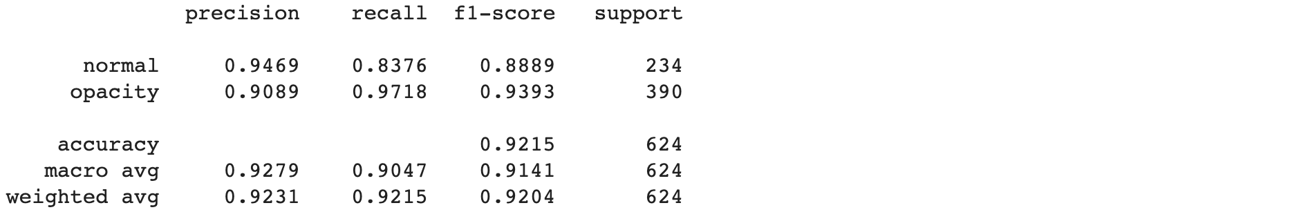
- Predict โรคปอดอักเสบด้วย Test Dataset เพื่อนำค่าความเชื่อมั่นมา Plot Histogram และแสดงการกระจายตัว รวมทั้ง ROC/AUC
y_score = model.predict(test_it)
y_score = y_score[:,0]
distribution_df = pd.DataFrame(data={'Score': y_score, 'Class': test_it.classes})
distribution_df.sample(5)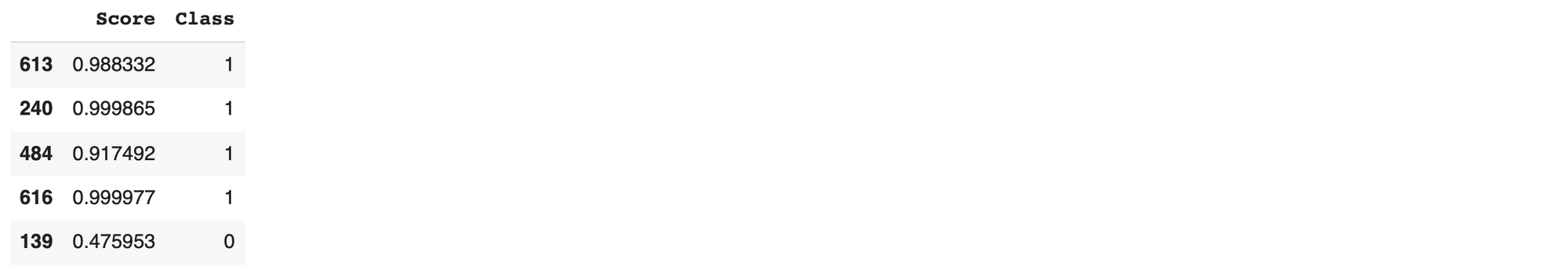
distribution_df.loc[distribution_df['Class'] == 1, 'Class'] = 'opacity'
distribution_df.loc[distribution_df['Class'] == 0, 'Class'] = 'normal'
distribution_df.sample(5)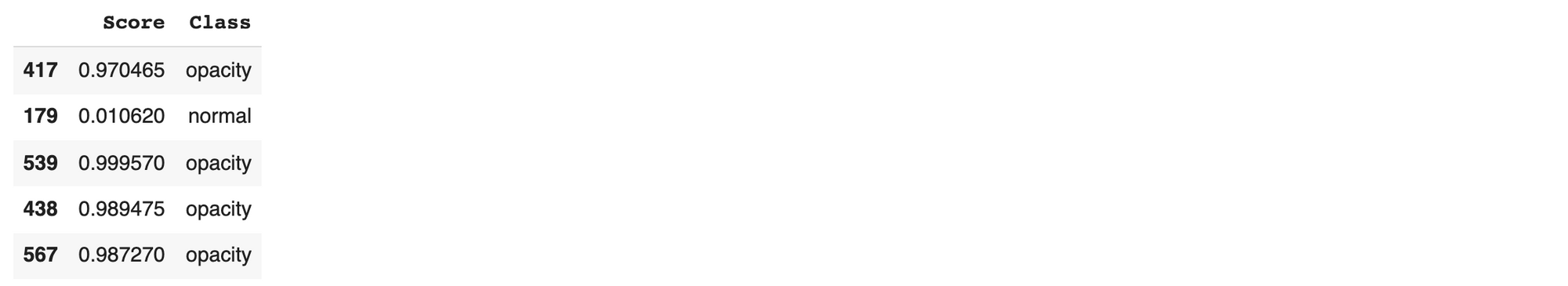
- Plot Histogram เพื่อแสดงการกระจายตัวของค่าความเชื่อมั่น
fig = px.histogram(distribution_df, x='Score', color='Class', nbins=50)
fig.update_layout(barmode='overlay')
fig.update_traces(opacity=0.85)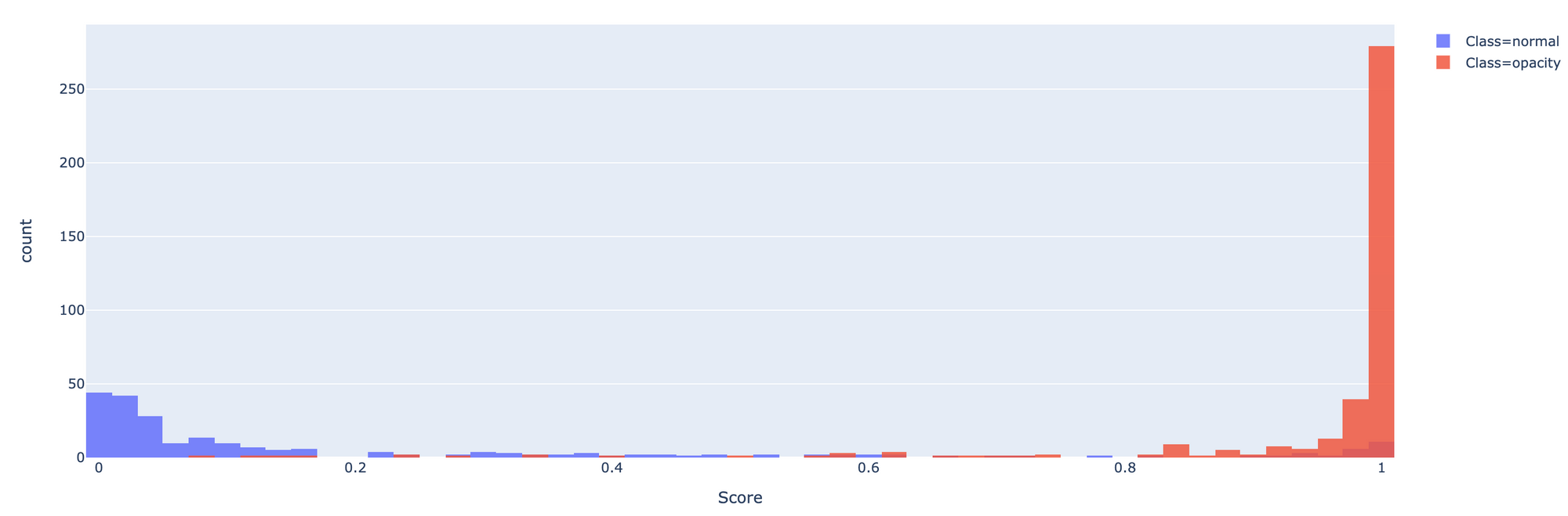
- คำนวณค่า True Positive Rate และ False Positive Rate ด้วยฟังก์ชัน roc_curve และนำ True Positive Rate และ False Positive Rate ที่ได้ไปคำนวณ AUC อีกทีด้วยฟังก์ชัน auc
fpr, tpr, threshold = roc_curve(test_it.classes, y_score)
roc_auc = auc(fpr, tpr)
roc_df = pd.DataFrame(data={'False Positive Rate': fpr, 'True Positive Rate': tpr, 'Threshold': threshold})
roc_df.head()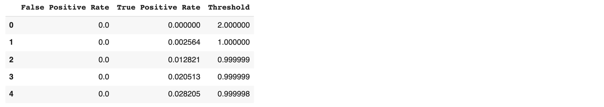
- นิยาม binary_roc_plot Function
def binary_roc_plot(roc_df, roc_auc):
    fig = px.area(
        data_frame=roc_df,
        x='False Positive Rate',
        y='True Positive Rate',
        hover_data=['Threshold'],
        title=f'ROC Curve (AUC={roc_auc:.4f})',
        width=700, height=500,
    )

    fig.add_shape(
        type='line', line=dict(dash='dash'),
        x0=0, x1=1, y0=0, y1=1
    )

    hovertemplate = 'False Positive Rate=%{x:.4f}<br>True Positive Rate=%{y:.4f}<br>Threshold=%{customdata[0]:.4f}'
    fig.update_traces(hovertemplate=hovertemplate)

fig.show()- Plot ROC Curve และ AUC
binary_roc_plot(roc_df, roc_auc)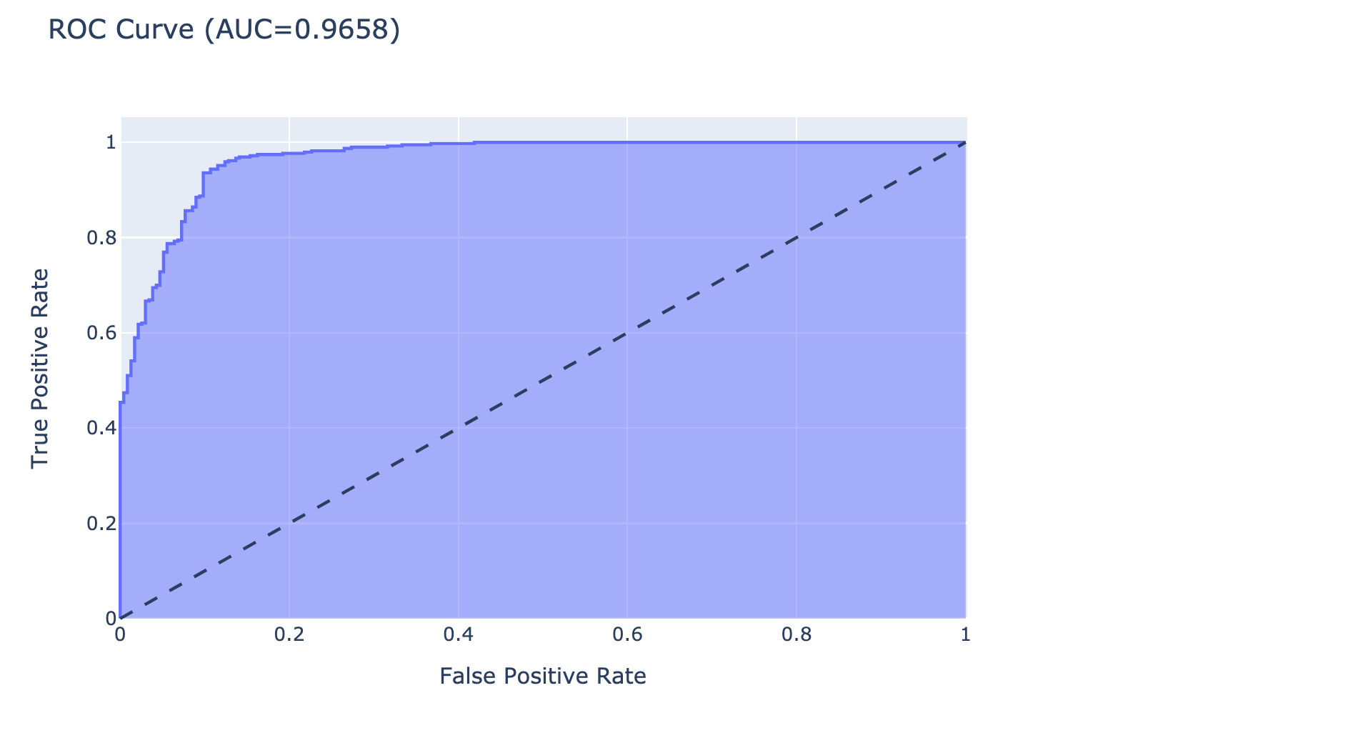
Multi-Class Classification
แม้ว่า Multi-Class Classification เป็น Model สำหรับข้อมูลที่มีผลเฉลยมากกว่า 2 Class ซึ่งผลลัพธ์ของ Model จะบอกถึงค่าความเชื่อมั่นในการทำนายของแต่ละ Class โดยค่าความเชื่อมั่นของทุกๆ Class รวมกันจะเท่ากับ 1.0 แต่เราก็สามารถนำมาประยุกต์ใช้กับปัญหาแบบ 2 Class เช่นการทำนายโรคปอดอักเสบได้เช่นเดียวกัน ซึ่งมีขั้นตอนในการพัฒนา Model แบบ Multi-Class ดังนี้
Load Dataset From Directory
- Load ภาพจาก Folder pneumonia-xray-images โดยใช้ ImageDataGenerator อีกครั้ง โดยกำหนด class_mode เป็น Categorical แทนที่จะเป็น Binary เพื่อกำหนด Format ของผลเฉลยเป็นแบบ One-hot
train_it = datagen.flow_from_directory('pneumonia-xray-images/train/',
                                       target_size=(img_rows, img_cols),
                                       batch_size=batch_size,
                                       class_mode='categorical',
                                       shuffle=True,
                                       color_mode='grayscale',
                                       seed=seed)
Found 4192 images belonging to 2 classes.
val_it = val_test_datagen.flow_from_directory('pneumonia-xray-images/val/',
                                              target_size=(img_rows, img_cols),
                                              batch_size=batch_size,
                                              class_mode='categorical',
                                              shuffle=False,
                                              color_mode='grayscale',
                                              seed=seed)
test_it = val_test_datagen.flow_from_directory('pneumonia-xray-images/test/',
                                               target_size=(img_rows, img_cols),
                                               batch_size=batch_size,
                                               class_mode='categorical',
                                               shuffle=False,
                                               color_mode='grayscale',
                                               seed=seed)
Found 1040 images belonging to 2 classes.
Found 624 images belonging to 2 classes.
Train Model
- เคลียร์ Tensorflow Session
tf.keras.backend.clear_session()- นิยาม Model แบบ Convolutional Neural Network (CNN) โดยกำหนด Activate Function แบบ Softmax และกำหนด Output Node = 2 ที่ Layer สุดท้าย
#Feature Extraction
model = tf.keras.Sequential()
model.add(tf.keras.layers.Input(shape=input_shape))
model.add(tf.keras.layers.Conv2D(32, kernel_size=(3, 3), activation='relu', input_shape=input_shape))
model.add(tf.keras.layers.MaxPooling2D(pool_size=(2, 2)))

model.add(tf.keras.layers.Conv2D(32, kernel_size=(3, 3), activation='relu'))
model.add(tf.keras.layers.MaxPooling2D(pool_size=(2, 2)))

model.add(tf.keras.layers.Conv2D(64, kernel_size=(3, 3), activation='relu'))
model.add(tf.keras.layers.MaxPooling2D(pool_size=(2, 2)))

model.add(tf.keras.layers.Conv2D(64, kernel_size=(3, 3), activation='relu'))
model.add(tf.keras.layers.MaxPooling2D(pool_size=(2, 2)))

#Image Classification
model.add(tf.keras.layers.Flatten())
model.add(tf.keras.layers.Dense(128, activation='relu'))
model.add(tf.keras.layers.Dense(64, activation='relu'))
model.add(tf.keras.layers.Dense(num_classes, activation='softmax'))
- Compile Model โดยกำหนด Loss Function แบบ Categorical Crossentropy
model.compile(loss='categorical_crossentropy', optimizer='adam', metrics=['accuracy'])
model.summary()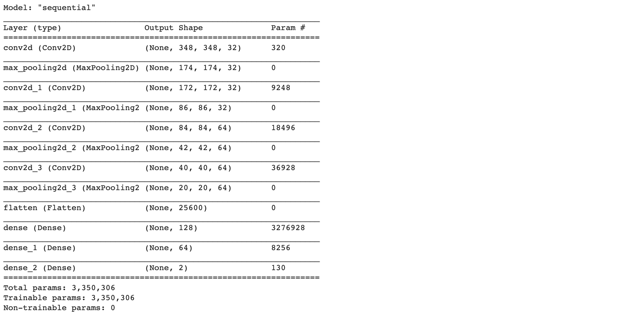
- Train Model โดยกำหนดให้ class_weight เท่ากับ cw และสุ่มภาพสำหรับ Train และ Validate
his = model.fit(
        train_it,
        validation_data=val_it,
        epochs=epochs,
        class_weight=cw,
        callbacks=callbacks_list,
        shuffle=True,
        steps_per_epoch=STEP_SIZE_TRAIN,
        validation_steps=STEP_SIZE_VALID)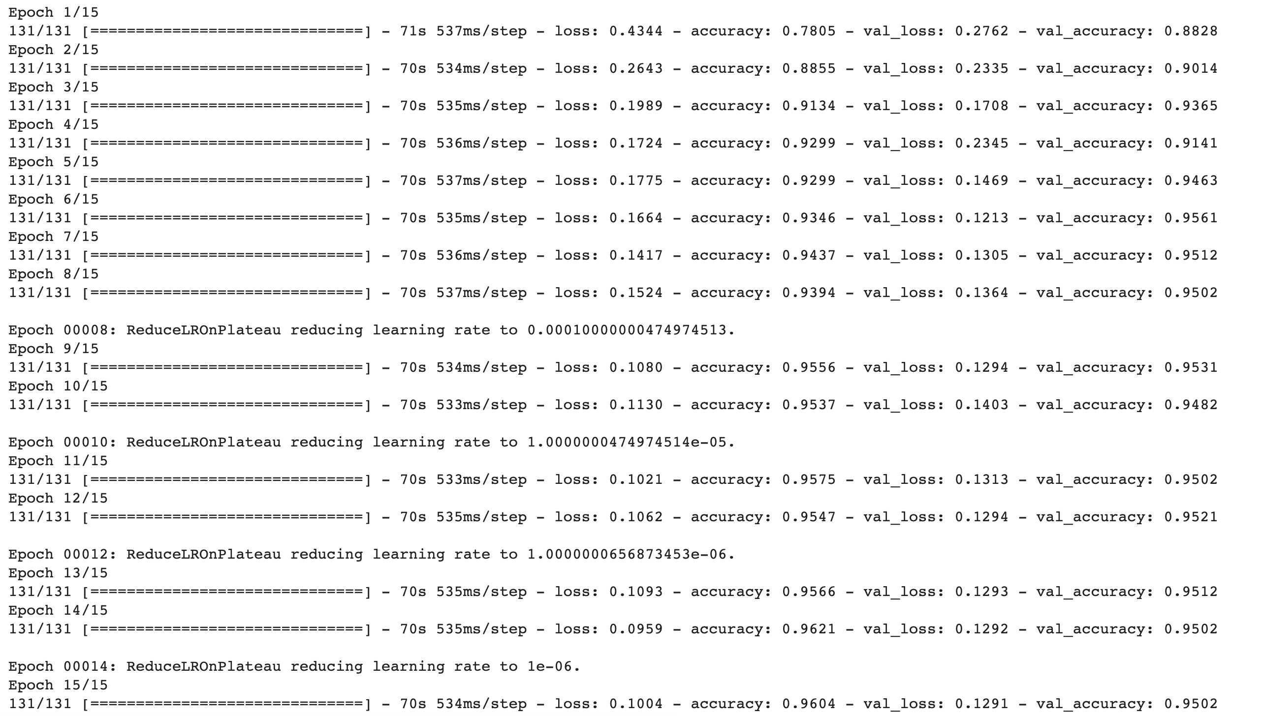
- Plot Loss
h1 = go.Scatter(y=his.history['loss'],
                    mode="lines",
                    line=dict(
                        width=2,
                        color='blue'),
                        name="loss"
                   )
h2 = go.Scatter(y=his.history['val_loss'],
                    mode="lines",
                    line=dict(
                        width=2,
                        color='red'),
                        name="val_loss"
                   )

data = [h1,h2]
layout1 = go.Layout(title='Loss',
                   xaxis=dict(title='epochs'),
                   yaxis=dict(title=''))
fig1 = go.Figure(data, layout=layout1)
plotly.offline.iplot(fig1)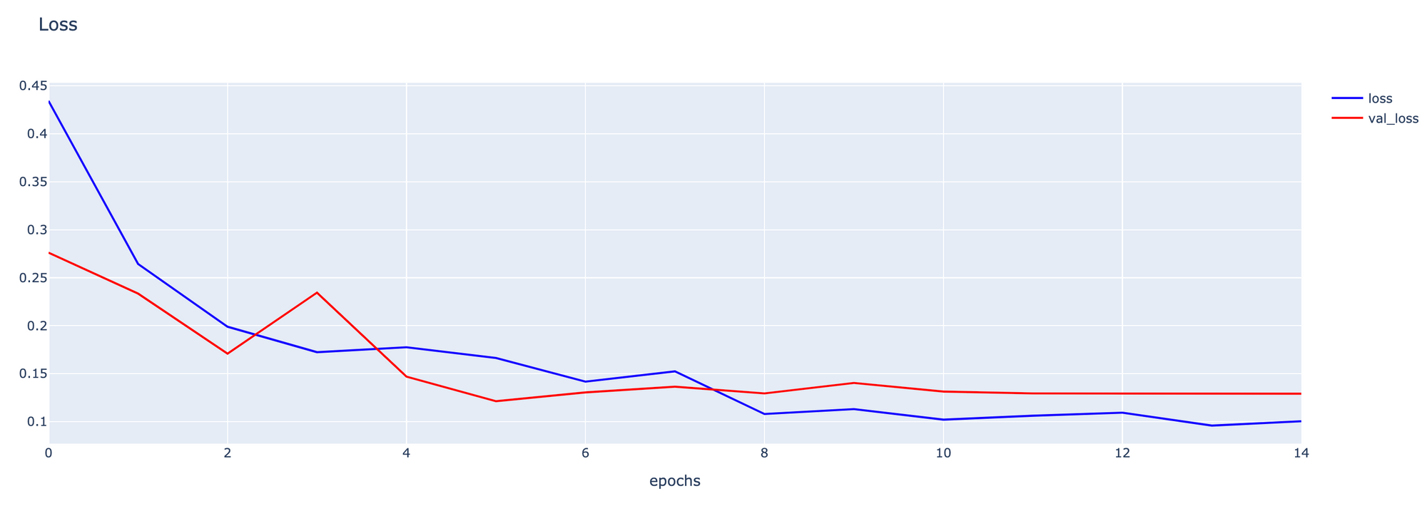
- Plot Accuracy
h1 = go.Scatter(y=his.history['accuracy'],
                    mode="lines", line=dict(
                    width=2,
                    color='blue'),
                    name="acc"
                   )
h2 = go.Scatter(y=his.history['val_accuracy'],
                    mode="lines", line=dict(
                    width=2,
                    color='red'),
                    name="val_acc"
                   )

data = [h1,h2]
layout1 = go.Layout(title='Accuracy',
                   xaxis=dict(title='epochs'),
                   yaxis=dict(title=''))
fig1 = go.Figure(data = data, layout=layout1)
plotly.offline.iplot(fig1)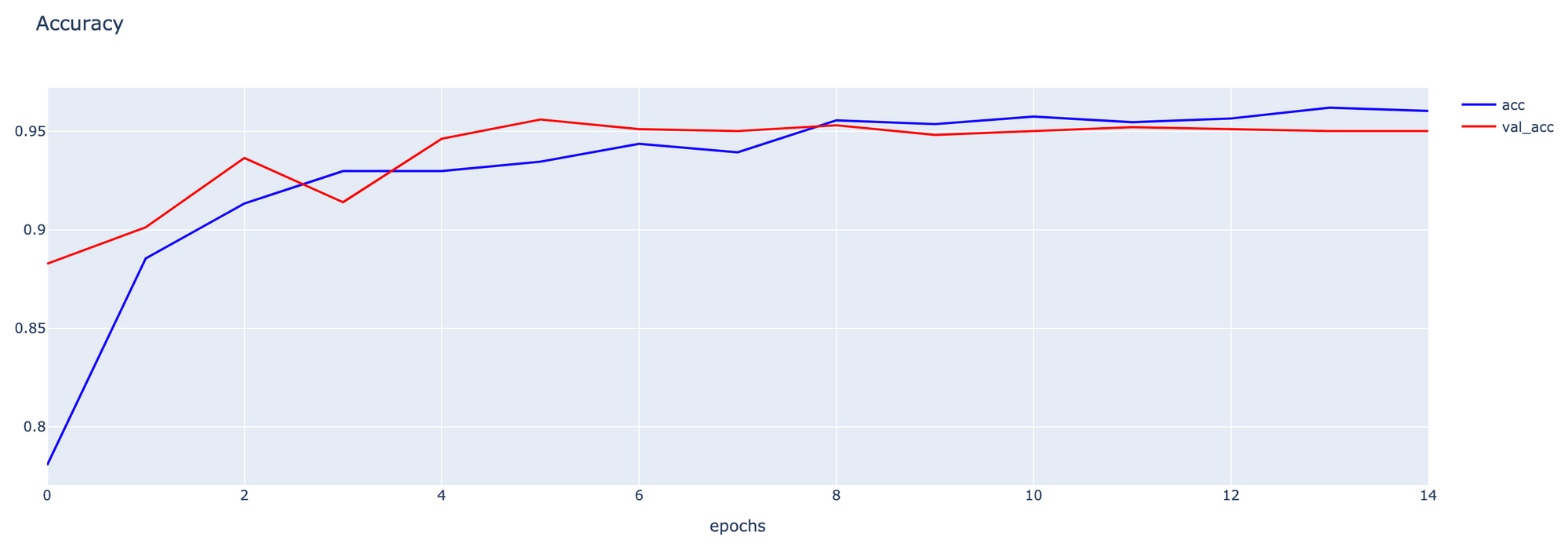
Multi-Class Classification Evaluation
- Predict โรคปอดอักเสบด้วย Test Dataset โดยใช้ค่าความเชื่อมั่นที่เกิดจากการใช้ Activate Function แบบ Softmax ในการคำนวณหมายเลข Class และคำนวณค่า ROC/AUC
predicted_score = model.predict(test_it, verbose=1)
predicted_classes = np.argmax(predicted_score, axis=1)
20/20 [==============================] - 4s 203ms/step
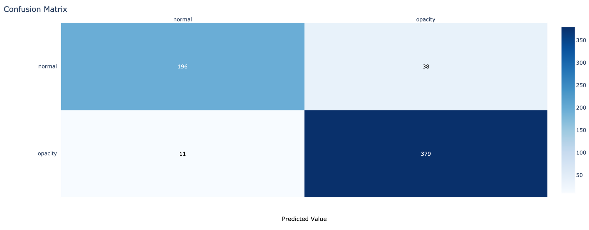
- คำนวณ Confusion Matrix
cm = confusion_matrix(test_it.classes, predicted_classes)
cm
- Plot Confusion Matrix
cm_plot(cm, labels)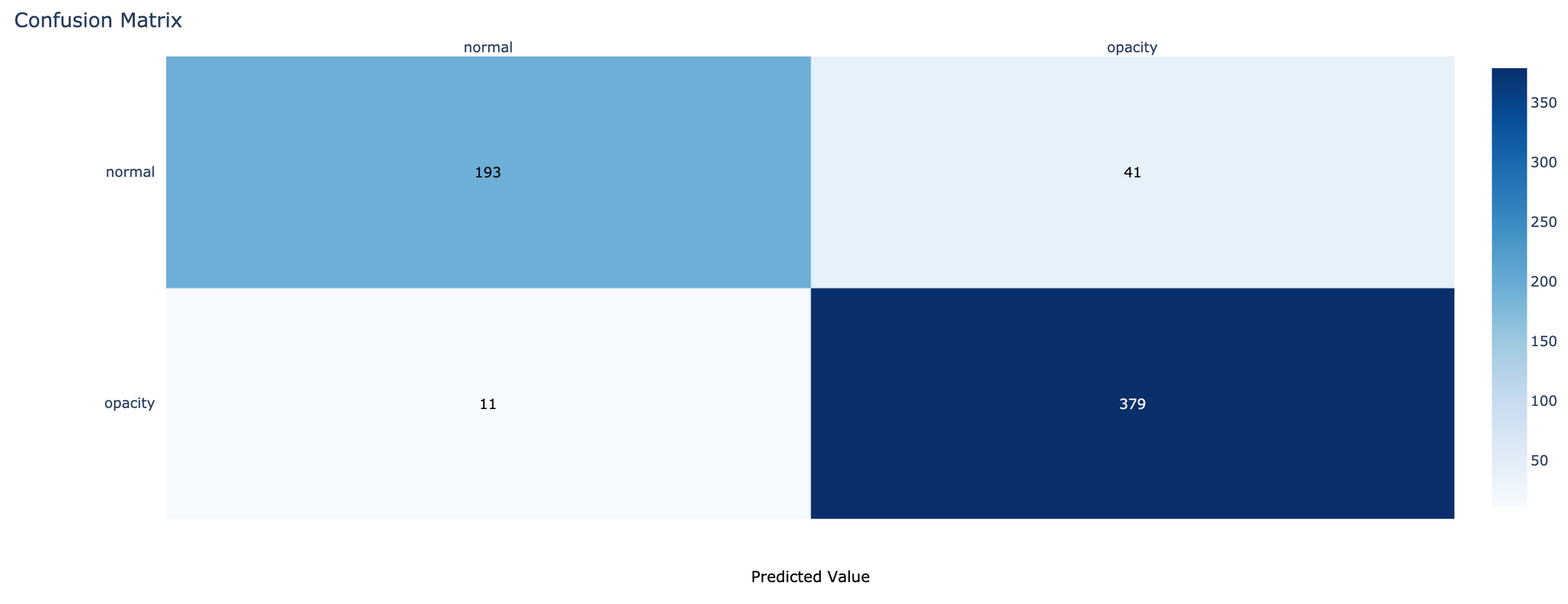
- คำนวณค่า Precision, Recall, F1-score
print(classification_report(test_it.classes, predicted_classes, target_names=labels, digits=4))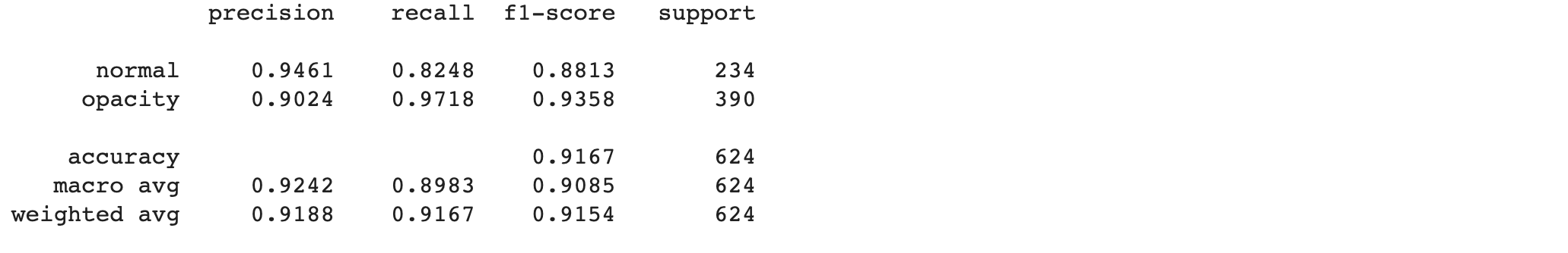
- Plot ROC/AUC ของ Binary Classification และ Multi-Class Classification พร้อมกัน
hovertemplate = 'False Positive Rate=%{x:.4f}<br>True Positive Rate=%{y:.4f}<br>Threshold=%{text:.4f}'
fig = go.Figure()
fig.add_shape(
    type='line', line=dict(dash='dash'),
    x0=0, x1=1, y0=0, y1=1
)

name = f"Binary Class, AUC={roc_auc:.4f}"
fig.add_trace(go.Scatter(x=roc_df['False Positive Rate'], y=roc_df['True Positive Rate'], name=name, mode='lines', text=roc_df['Threshold'], hovertemplate=hovertemplate))

multi_class_fpr, multi_class_tpr, multi_class_threshold = roc_curve(test_it.classes, predicted_score[:, 1])
multi_class_roc_auc = auc(multi_class_fpr, multi_class_tpr)
name = f"Multi-Class, AUC={multi_class_roc_auc:.4f}"
fig.add_trace(go.Scatter(x=multi_class_fpr, y=multi_class_tpr, name=name, mode='lines', text=multi_class_threshold, hovertemplate=hovertemplate))

fig.update_layout(
    title='ROC Curve and AUC',
    xaxis_title='False Positive Rate',
    yaxis_title='True Positive Rate',
)

fig.show()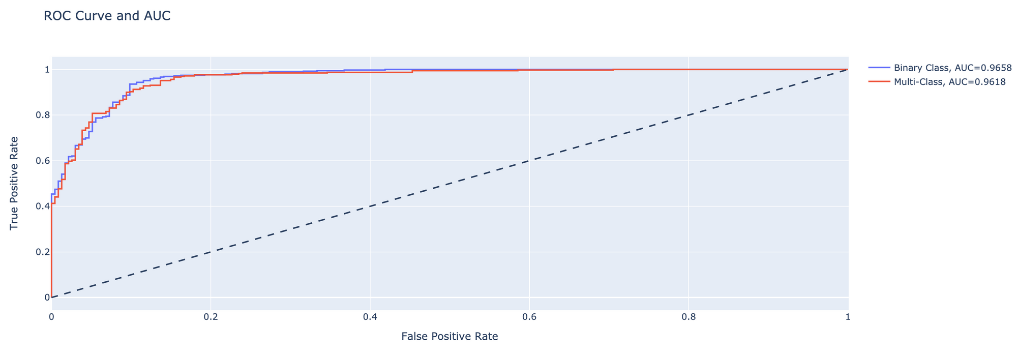
จากการทดลอง Train Model ทั้งหมด 15 Epoch พบว่า Model แบบ Binary Classification มีความสามารถในการแยกภาพปอดอักเสบออกจากภาพปอดปกติได้ดีกว่า Model แบบ Multi-Class Classification โดยมีค่า AUC เท่ากับ 0.9658
นอกจากจะสามารถแยกภาพปอดอักเสบได้ดีกว่าแล้ว ข้อดีของ Binary Classification อีกอย่างหนึ่งคือ เราสามารถปรับลดค่า Threshold เพื่อลดผลการทำนายแบบ False Negative ได้ (ต้องมีการ Trade-off กับ False Positive Rate) สำหรับกรณีที่เราซีเรียสเรื่องปอดอักเสบ แต่ Model ทำนายผิดว่าปอดไม่อักเสบ
อย่างไรก็ตามการจะบอกว่าประสิทธิภาพของ Model แบบไหนดีกว่ากันจริงๆ คงต้องมีการเพิ่มจำนวน Epoch ในการ Train และปรับ Parameter ต่างๆ ให้ละเอียดยิ่งขึ้นครับ