บทความโดย ผศ.ดร.ณัฐโชติ พรหมฤทธิ์
ภาควิชาคอมพิวเตอร์
คณะวิทยาศาสตร์
มหาวิทยาลัยศิลปากร

สำหรับผู้อ่านบางท่านที่เริ่มต้นศึกษา Machine Learning Model อาจจะเคยสับสนกับคำว่า Parameter และ Hyperparameter กันมาบ้าง โดย Parameter จะเป็นตัวแปร (Variable) ที่อยู่ภายใน Model เช่น Weight และ Bias ซึ่งจะถูกประมาณค่าโดยอัตโนมัติจาก Dataset ที่ใช้สอนโดยตรง ขณะที่ Hyperparameter จะเป็นตัวแปรภายนอก Model เช่น Learning Rate, Droupout Rate, Batch Size ฯลฯ ซึ่งไม่ได้เกิดจากการประมาณค่าโดยตรงจาก Dataset

Learning Rate เป็น Hyperparameter ที่สำคัญตัวหนึ่ง ที่มีหน้าที่ในการปรับขนาดของ Error ในแต่ครั้งของการปรับปรุง Weight และ Bias ด้วย Back-propagation Algorithm ดังสมการต่อไปนี้

Update w = w - Learning_Rate*Error_at_w

ซึ่งการปรับเปลี่ยน Learning Rate จะมีผลกระทบกับประสิทธิภาพของ Model เป็นอย่างมาก ถ้าให้เลือกว่าจะปรับจูน Hyperparameter ตัวไหนก่อน Learning Rate คงเป็น Hyperparameter ตัวแรกๆ ที่ควรจะพิจารณาครับ

ในบทความนี้ผู้อ่านจะได้ทำความเข้าใจผลลัพธ์ที่เกิดจากการใช้เทคนิคในการปรับค่า Learning Rate และ Momentum ครับ

Impact of Learning Rate

เราจะใช้ Learning Rate ควบคุมความเร็วในการปรับตัวของ Model ต่อปัญหาที่มันจะต้องแก้ ซึ่งการกำหนด Learning Rate ขนาดเล็ก จะทำให้ในการ Train Model แต่ละรอบมันจะปรับปรุง Weight และ Bias ทีละนิด จึงต้องการจำนวน Epoch หลาย Epoch ขณะที่การกำหนด Learning Rate ขนาดใหญ่ จะทำให้ในการ Train แต่ละรอบจะมีการปรับปรุง Weight และ Bias อย่างรวดเร็ว จึงต้องการจำนวน Epoch ที่น้อยกว่า

ใน Keras Framework ผู้อ่านสามารถกำหนดค่า Learning Rate เริ่มต้น ผ่านทาง Stochastic Gradient Descent Algorithm แบบต่างๆ อย่างเช่น SGD, AdaGrad (Adaptive Gradient Algorithm), RMSprop (Root Mean Square Propagation) หรือ Adam (Adaptive Moment Estimation) ฯลฯ ซึ่งเราเรียก Algorithm เหล่านี้ว่า Optimizer

โดยเราจะสร้าง Neural Network อย่างง่ายเพื่อจำแนกข้อมูล 3 Class และทดลองปรับ Learning Rate ตั้งแต่ 1.0 ถึง 0.0000001 ผ่าน SGD Optimizer (Optimizer พื้นฐานที่เราสามารถกำหนดวิธีการปรับ Learning Rate ได้ด้วยตัวเอง)

แต่ก่อนอื่นเราจะใช้ make_blobs() Function ของ scikit-learn Library ในการสร้าง Dataset ขนาด 2 มิติ ที่มี 3 Class ตามตัวอย่างด้านล่าง

import tensorflow as tf
K = tf.keras.backend
Callback = tf.keras.callbacks.Callback
ReduceLROnPlateau = tf.keras.callbacks.ReduceLROnPlateau

to_categorical = tf.keras.utils.to_categorical

from sklearn.datasets import make_blobs
from matplotlib import pyplot
from numpy import where

from sklearn.model_selection import train_test_split

import pandas as pd
import plotly.express as px
from plotly.subplots import make_subplots
import plotly.graph_objects as go
import plotly

x, y = make_blobs(n_samples=3000, centers=3, n_features=2, cluster_std=2, random_state=2)

แล้วแยก Dataset เป็น 2 ส่วน สำหรับการ Train 60% และสำหรับการ Validate อีก 40%

x_train, x_val, y_train, y_val = train_test_split(x, y, test_size=0.4, shuffle= True)

x_train.shape, x_val.shape, y_train.shape, y_val.shape

((1800, 2), (1200, 2), (1800,), (1200,))

นำ Dataset ส่วนที่ Train มาแปลงเป็น DataFrame โดยเปลี่ยนชนิดข้อมูลใน Column "class" เป็น String เพื่อทำให้สามารถแสดงสีแบบไม่ต่อเนื่องได้ แล้วนำไป Plot

x_train_pd = pd.DataFrame(x_train, columns=['x', 'y'])
y_train_pd = pd.DataFrame(y_train, columns=['class'])

df = pd.concat([x_train_pd, y_train_pd], axis=1)
df["class"] = df["class"].astype(str)

fig = px.scatter(df, x="x", y="y", color="class")
fig.show()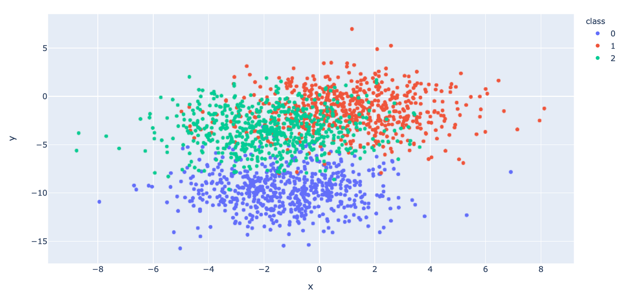

เราจะเข้ารหัสผลเฉลย แบบ One-Hot Encoder เพื่อที่ว่าเมื่อ Model มีการ Pridict ว่าเป็น Class ไหน มันจะให้ค่าความมั่นใจ (Confidence) กลับมาด้วยทุกครั้ง

y_train = to_categorical(y_train)
y_val = to_categorical(y_val)

นิยาม create_model1 Function

def create_model1(learning_rates):
    model = tf.keras.Sequential()
    model.add(tf.keras.layers.Dense(50, input_dim=2, activation='relu', kernel_initializer='he_uniform'))
    model.add(tf.keras.layers.Dense(3, activation='softmax', kernel_initializer='he_uniform'))
    
    opt = tf.keras.optimizers.SGD(lr=learning_rates)
    model.compile(loss='categorical_crossentropy', optimizer=opt, metrics=['accuracy'])
    
    return model

Train Model และ Plot กราฟ accuracy และ val_accuracy

learning_rates = [1.0, 0.1, 0.01, 0.001, 0.0001, 0.00001, 0.000001, 0.0000001]

fig = make_subplots(
    rows=4, cols=2,
    subplot_titles=('lr=1.0', 'lr=0.1', 'lr=0.01', 'lr=0.001', 'lr=0.0001', 'lr=0.00001', 'lr=0.000001', 'lr=0.0000001')
)

for i in range(len(learning_rates)):
    model = create_model1(learning_rates[i])
    
    row = (i//2)+1
    col = (i%2)+1
    history = model.fit(x_train, y_train, validation_data=(x_val, y_val), epochs=200, verbose=0)
    
    fig.add_trace(go.Scatter(y=history.history['accuracy'], line=dict(color='blue')), row=row, col=col)
    fig.add_trace(go.Scatter(y=history.history['val_accuracy'], line=dict(color='red')), row=row, col=col)
    
    fig.update_xaxes(title_text='Epochs', showgrid=False, row=row, col=col)
    fig.update_yaxes(title_text='Accuracy', showgrid=False, row=row, col=col)
    
fig.update_layout(title_text='Impact of Learning Rate', height=750, showlegend=False)   

เมื่อ Train เสร็จแล้ว ผู้อ่านจะเห็นกราฟ Accuracy หรือ Learning Curve ของ Model ดังภาพ

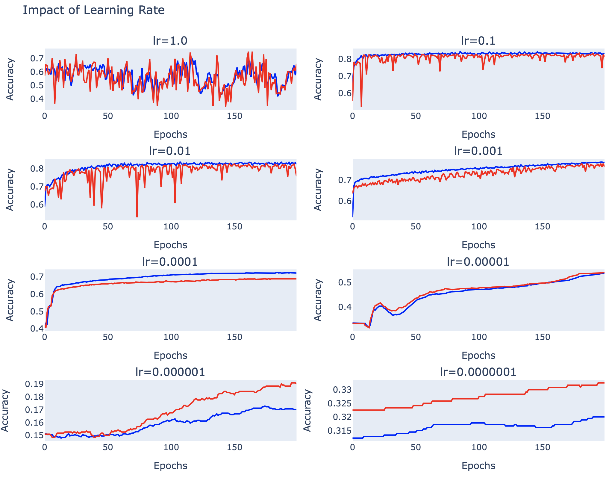
จากภาพด้านบน จะเห็นว่าที่ lr = 1.0 กราฟ Accuracy (สีน้ำเงิน) และ Validate Accuracy (สีแดง) จะมีการแกว่งขึ้นลงอย่างมาก และที่ lr = 0.000001 และ 0.0000001, Model มีการเรียนรู้ต่ำ ขณะที่ที่ lr = 0.1, 0.01 และ 0.001  Model ประสบความสำเร็จในการเรียนรู้ค่อนข้างมาก ซึ่งที่ lr = 0.1 Model มีอัตราการเรียนรู้สูงที่สุด คือ มี Accuracy สูงกว่า 80% ตั้งแต่ Epoch ต้นๆ อย่างไรก็ตามเพื่อจะให้ผู้อ่านเห็นว่าเทคนิคต่างๆ สำหรับการปรับค่า Learning Rate จะสามารถเพิ่มประสิทธิภาพให้ Model อย่างไรบ้าง ในหัวข้อถัดๆ ไป จะมีการกำหนดค่า Learning Rate ไว้ที่ 0.01 ครับ

Momentum

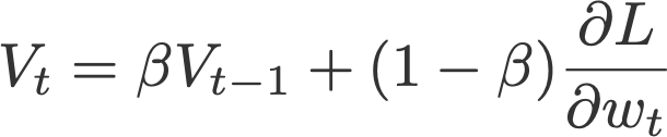
Momentum (β) เป็นเทคนิคในการลดการแกว่งของ Learning Curves พร้อมกับเร่งอัตราการเรียนรู้ของ Model ให้เร็วขึ้น โดยใช้ Velocity (ความเร็ว) ของรอบก่อนหน้า และ Error ในรอบปัจจุบันเพื่อปรับปรุง Weight และ Bias ด้วยค่าน้ำหนักตามที่กำหนด (ใช้ β ในการปรับ Error แทนที่จะใช้ Learning Rate) ซึ่งโดยปกติจะมีการให้น้ำหนัก Velocity ในรอบก่อนหน้ามากกว่า Error ในรอบปัจจุบัน เช่น ถ้ากำหนด β = 0.9 แสดงว่าเราจะให้น้ำหนัก Velocity ในรอบก่อนหน้าเท่ากับ 0.9 และ Error ในรอบปัจจุบันเท่ากับ 0.1 ดังสมการต่อไปนี้

where

นิยาม create_model2 Function โดยกำหนด lr = 0.01

def create_model2(momentum):
    model = tf.keras.Sequential()
    model.add(tf.keras.layers.Dense(50, input_dim=2, activation='relu', kernel_initializer='he_uniform'))
    model.add(tf.keras.layers.Dense(3, activation='softmax', kernel_initializer='he_uniform'))
    
    opt = tf.keras.optimizers.SGD(lr=0.01, momentum=momentum)
    model.compile(loss='categorical_crossentropy', optimizer=opt, metrics=['accuracy'])
    
    return model

Train Model และ Plot กราฟ accuracy และ val_accuracy

momentums = [0.0, 0.5, 0.9, 0.99]

fig = make_subplots(
    rows=4, cols=2,
    subplot_titles=('Momentum=0.0', 'Momentum=0.5', 'Momentum=0.9', 'Momentum=0.99')
)

for i in range(len(momentums)):
    model = create_model2(momentums[i])
    
    row = (i//2)+1
    col = (i%2)+1
    history = model.fit(x_train, y_train, validation_data=(x_val, y_val), epochs=200, verbose=0)
    
    fig.add_trace(go.Scatter(y=history.history['accuracy'], line=dict(color='blue')), row=row, col=col)
    fig.add_trace(go.Scatter(y=history.history['val_accuracy'], line=dict(color='red')), row=row, col=col)
    
    fig.update_xaxes(title_text='Epochs', showgrid=False, row=row, col=col)
    fig.update_yaxes(title_text='Accuracy', showgrid=False, row=row, col=col)
    
fig.update_layout(title_text='Impact of Momentum', height=750, showlegend=False)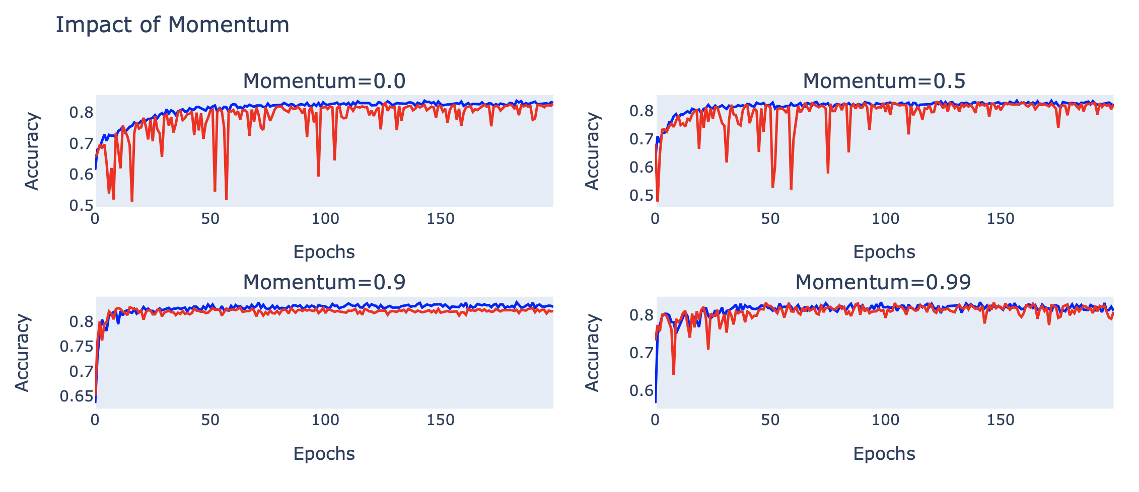   

จากภาพด้านบน จะเห็นว่าที่ momentum (β) = 0.9 Learning Curves ของ Model มีการแกว่งน้อยกว่า รวมทั้งมีอัตราการเรียนรู้ที่เร็วขึ้นกว่าตอนที่ไม่ได้ใช้ momentum อย่างเห็นได้ชัด

Learning Rate Decay

นอกจากนี้เรายังสามารถเพิ่มประสิทธิภาพของ Model ได้โดยการค่อย ๆ ลด Learning Rate (Learning Rate Decay) ในแต่ละ Epoch ในอัตราที่เหมาะสม ดังเช่นในตัวอย่างต่อไปนี้

def decay_lrate(initial_lrate, decay, iteration):
    return initial_lrate * (1.0 / (1.0 + decay * iteration))

data = []
decays = [0.1, 0.01, 0.001, 0.0001]
learning_rate = 0.01
EPOCH = 200
colors = ['red', 'green', 'blue', 'orange']

for i, decay in enumerate(decays):
    learning_rates = [decay_lrate(learning_rate, decay, i) for i in range(EPOCH)]
    
    h = go.Scatter(y=learning_rates, 
                     mode="lines",
                     line=dict(
                         width=2,
                         color=colors[i]),
                     name=str(decay))
    
    data.append(h)
    
layout1 = go.Layout(title='Learning Rate',
                   xaxis=dict(title='Epochs'),
                   yaxis=dict(title=''))
fig1 = go.Figure(data, layout=layout1)
plotly.offline.iplot(fig1)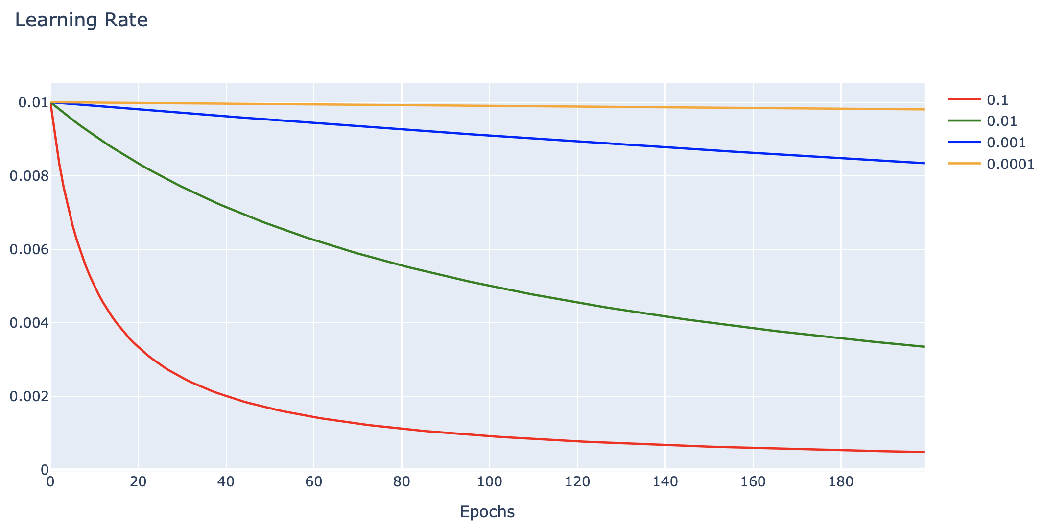

นิยาม create_model3 Function โดยกำหนด lr = 0.01

def create_model3(decay):
    model = tf.keras.Sequential()
    model.add(tf.keras.layers.Dense(50, input_dim=2, activation='relu', kernel_initializer='he_uniform'))
    model.add(tf.keras.layers.Dense(3, activation='softmax', kernel_initializer='he_uniform'))
    
    opt = tf.keras.optimizers.SGD(lr=0.01, decay=decay)
    model.compile(loss='categorical_crossentropy', optimizer=opt, metrics=['accuracy'])
    
    return model

Train Model และ Plot กราฟ accuracy และ val_accuracy

fig = make_subplots(
    rows=2, cols=2,
    subplot_titles=('Decay=0.1', 'Decay=0.01', 'Decay=0.001', 'Decay=0.0001')
)

for i in range(len(decays)):
    model = create_model3(decays[i])
    
    row = (i//2)+1
    col = (i%2)+1
    history = model.fit(x_train, y_train, validation_data=(x_val, y_val), epochs=200, verbose=0)
    
    fig.add_trace(go.Scatter(y=history.history['accuracy'], line=dict(color='blue')), row=row, col=col)
    fig.add_trace(go.Scatter(y=history.history['val_accuracy'], line=dict(color='red')), row=row, col=col)
    
    fig.update_xaxes(title_text='Epochs', showgrid=False, row=row, col=col)
    fig.update_yaxes(title_text='Accuracy', showgrid=False, row=row, col=col)
    
fig.update_layout(title_text='Impact of Decay', height=750, showlegend=False)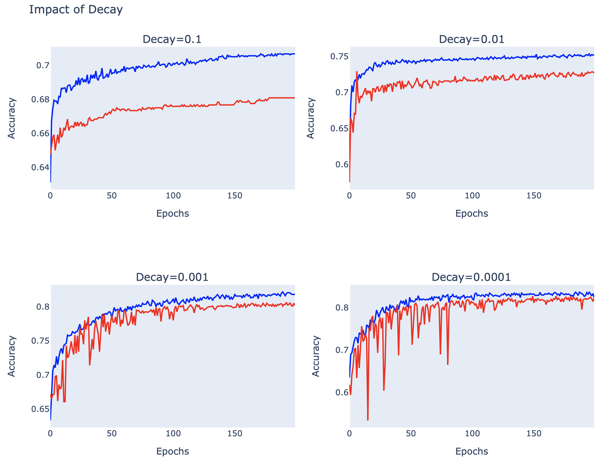   

จากภาพจะเห็นว่าที่ decay = 0.001 และ 0.0001, เส้นกราฟของ Model ในรอบหลัง มีการแกว่งน้อยกว่ารอบแรกๆ รวมทั้งมีค่า Accuracy ที่สูงกว่าตอนที่ยังไม่ได้ใช้ decay ครับ

Drop Learning Rate on Plateau

ในกรณีที่ Loss Value ไม่ลดลงเป็นระยะเวลาหนึ่ง เราจะเรียกสถานการณ์นี้ว่าการเจอที่ราบสูง (Plateau) เราอาจจะใช้เทคนิคการปรับลดค่า Learning Rate ด้วยการคูณกับค่า factor เช่น กำหนดให้  factor = 0.1, Learning Rate = 0.01 เมื่อ Loss Value ไม่ลดลง 5 Epoch เมื่อเปรียบเทียบกับ Loss Value น้อยที่สุด (patience=5) Learning Rate จะถูกปรับลดลงเป็น 0.001 (0.1*0.01) ตามตัวอย่างต่อไปนี้

นิยาม create_model4 Function โดยกำหนด lr = 0.01

class LearningRateMonitor(Callback):
    def on_train_begin(self, logs={}):
        self.learning_rates = list()
 
    def on_epoch_end(self, epoch, logs={}):
        optimizer = self.model.optimizer
        learning_rate = float(K.get_value(self.model.optimizer.lr))
        self.learning_rates.append(learning_rate)

def create_model4(patience):
    model = tf.keras.Sequential()
    model.add(tf.keras.layers.Dense(50, input_dim=2, activation='relu', kernel_initializer='he_uniform'))
    model.add(tf.keras.layers.Dense(3, activation='softmax', kernel_initializer='he_uniform'))
    
    opt = tf.keras.optimizers.SGD(lr=0.01, decay=decay)
    model.compile(loss='categorical_crossentropy', optimizer=opt, metrics=['accuracy'])
    
    rlrp = ReduceLROnPlateau(monitor='val_loss', factor=0.1, patience=patience)
    lrm = LearningRateMonitor()
    

    return model, rlrp, lrm

Train Model และ Plot กราฟ Learning Rate, val_loss และ val_accuracy

patiences = [2, 5, 10, 15]

learning_rate_list=[]
accuracy_list=[]
loss_list=[]

for i in range(len(patiences)):
    model, rlrp, lrm = create_model4(patiences[i])
    
    history = model.fit(x_train, y_train, validation_data=(x_val, y_val), epochs=200, verbose=0, callbacks=[rlrp, lrm])
    lrm.learning_rates
    
    learning_rate_list.append(lrm.learning_rates)
    accuracy_list.append(history.history['val_accuracy'])
    loss_list.append(history.history['val_loss'])
    

def patiences_plot(y, title_text):
    fig = make_subplots(
        rows=2, cols=2,
        subplot_titles=('Patience=2', 'Patience=5', 'Patience=10', 'Patience=15')
    )

    for i in range(len(patiences)):
        model = create_model4(patiences[i])

        row = (i//2)+1
        col = (i%2)+1
        fig.add_trace(go.Scatter(y=y[i], line=dict(color='red')), row=row, col=col)
        fig.update_xaxes(title_text='Epochs', showgrid=False, row=row, col=col)
        fig.update_yaxes(title_text=title_text, showgrid=False, row=row, col=col)

    fig.update_layout(title_text='Impact of Patience', height=750, showlegend=False)
    fig.show()

patiences_plot(learning_rate_list, 'Learning Rate')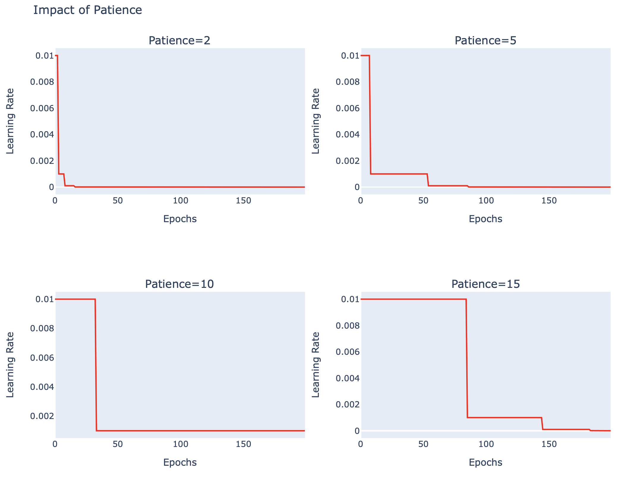

patiences_plot(loss_list, 'val_loss')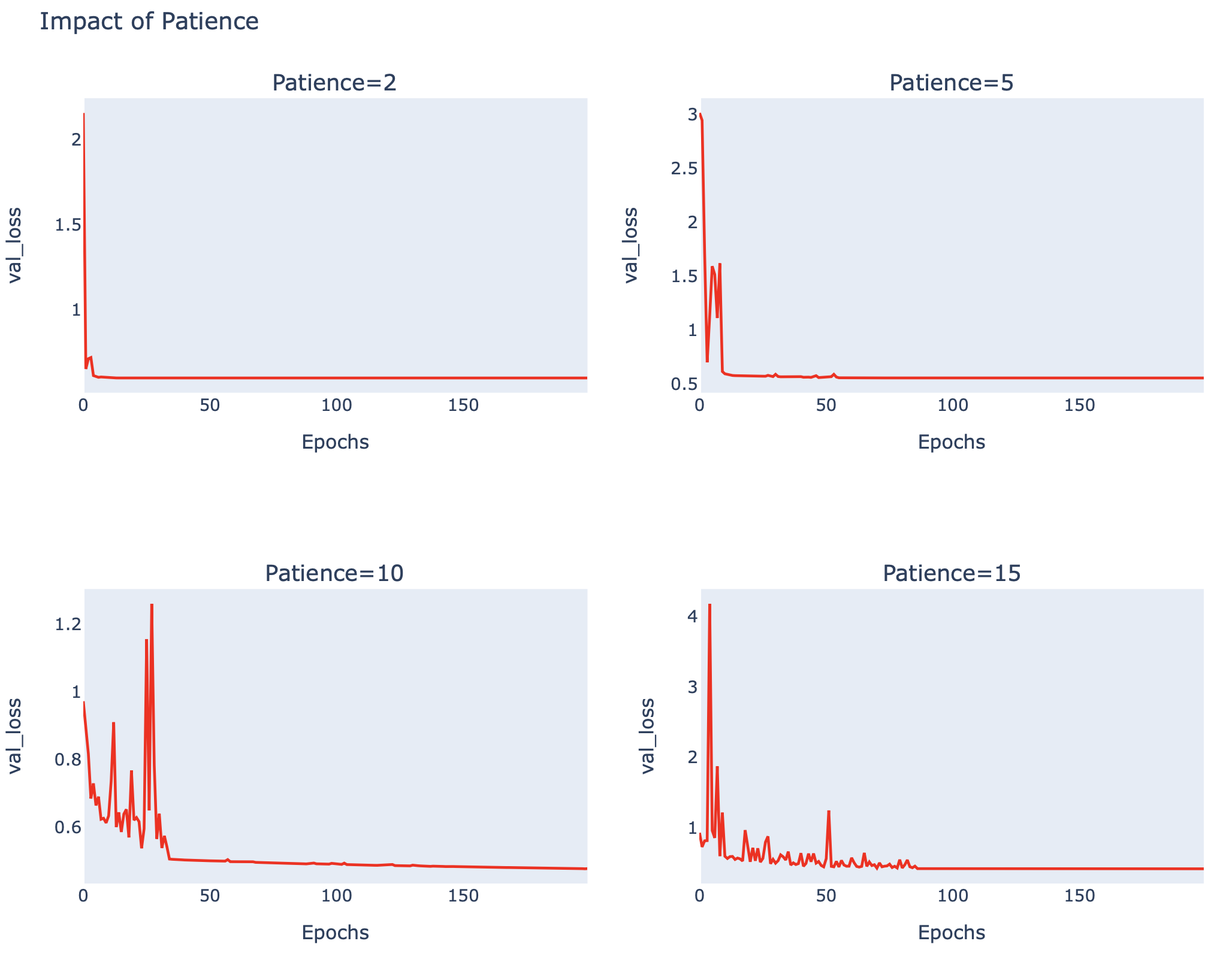

patiences_plot(accuracy_list, 'val_accuracy')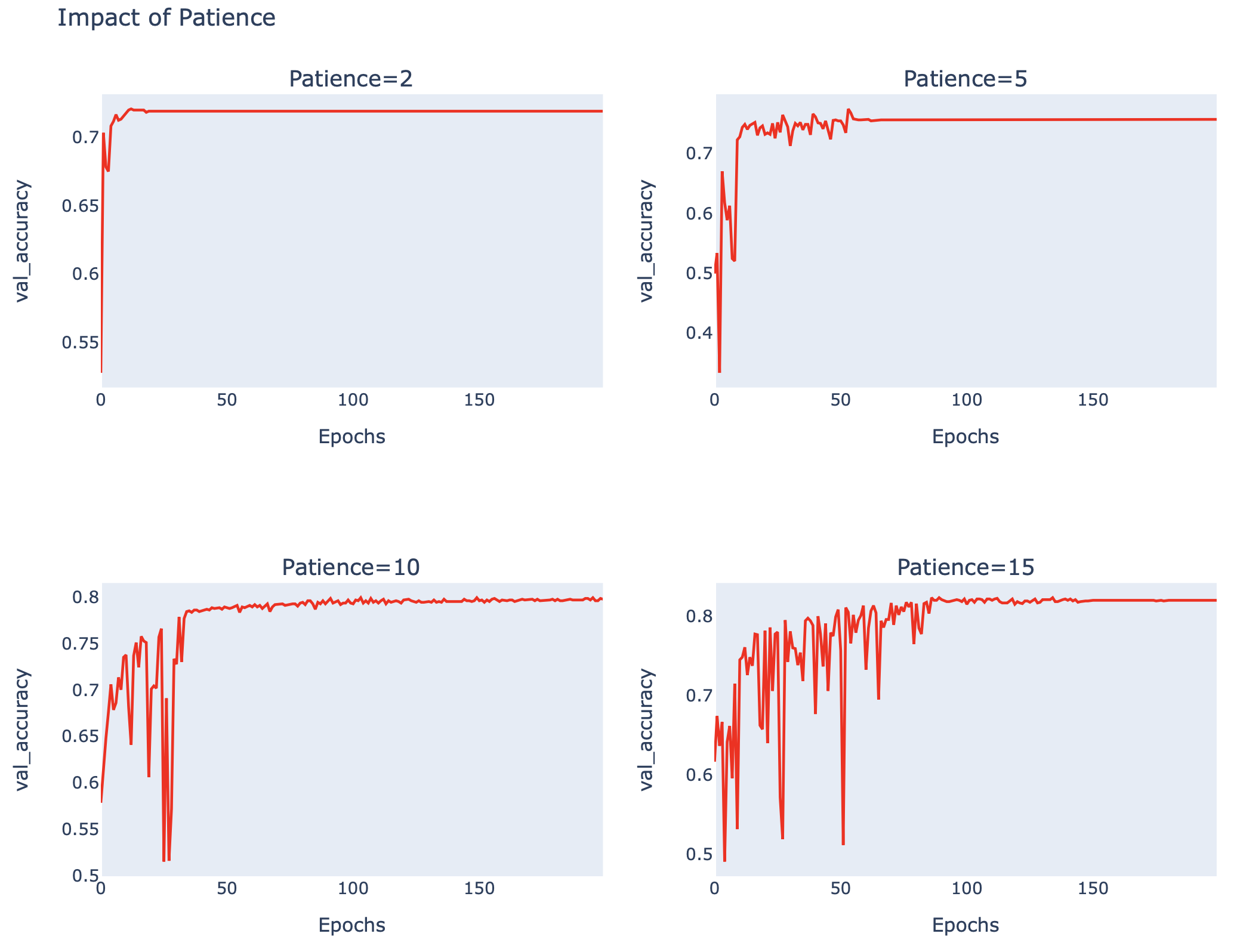

จากภาพด้านบน จะเห็นว่าที่ patience = 10, Loss Value ลดลงจนน้อยกว่า 0.4 ขณะที่ Accuracy เพิ่มขึ้นมากกว่า 80%

Adaptive Learning Rates Gradient Descent

ในตอนสุดท้ายของบทความ เราจะเปรียบเทียบ Adaptive Learning Rate Algorithm ได้แก่ AdaGrad (Adaptive Gradient Algorithm), RMSprop (Root Mean Square Propagation) และ Adam (Adaptive Moment Estimation) กับ Optimizer พื้นฐาน (SGD Optimizer) ครับ

นิยาม create_model5 Function

def create_model5(optimizer):
    model = tf.keras.Sequential()
    model.add(tf.keras.layers.Dense(50, input_dim=2, activation='relu', kernel_initializer='he_uniform'))
    model.add(tf.keras.layers.Dense(3, activation='softmax', kernel_initializer='he_uniform'))
    
    model.compile(loss='categorical_crossentropy', optimizer=optimizer, metrics=['accuracy'])
    
    return model

Train Model และ Plot กราฟ Accuracy

optimizers = ['sgd', 'rmsprop', 'adagrad', 'adam']

fig = make_subplots(
    rows=2, cols=2,
    subplot_titles=('Optimizer=sgd', 'Optimizer=rmsprop', 'Optimizer=adagrad', 'Optimizer=adam')
)

for i in range(len(optimizers)):
    model = create_model5(optimizers[i])
    
    row = (i//2)+1
    col = (i%2)+1
    history = model.fit(x_train, y_train, validation_data=(x_val, y_val), epochs=200, verbose=0)
    
    fig.add_trace(go.Scatter(y=history.history['accuracy'], line=dict(color='blue')), row=row, col=col)
    fig.add_trace(go.Scatter(y=history.history['val_accuracy'], line=dict(color='red')), row=row, col=col)
    
    fig.update_xaxes(title_text='Epochs', showgrid=False, row=row, col=col)
    fig.update_yaxes(title_text='Accuracy', showgrid=False, row=row, col=col)
    
fig.update_layout(title_text='Impact of Optimizer', height=750, showlegend=False)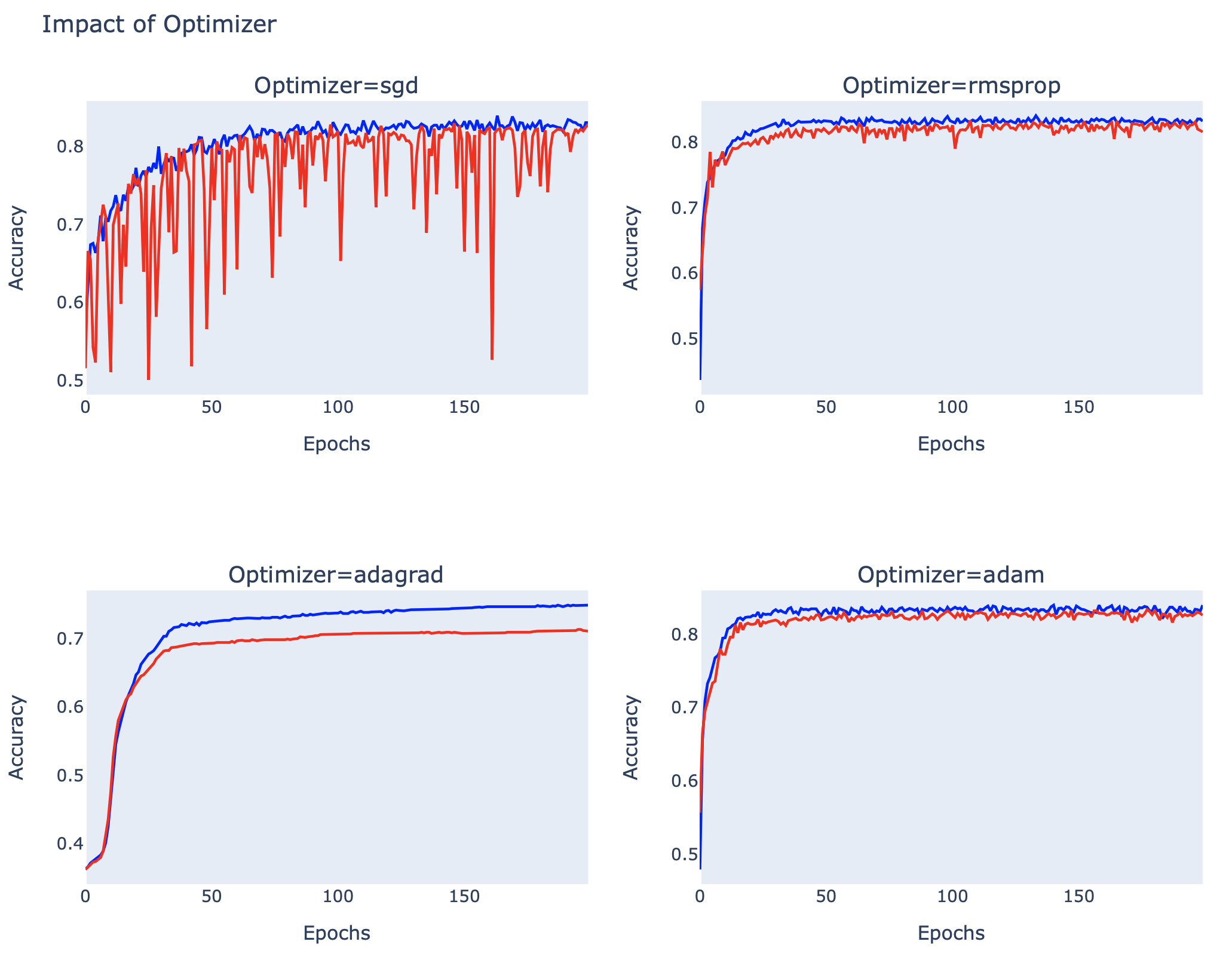   

หมายเหตุ  บางส่วนของตัวอย่างในการทดลองของบทความนี้ดัดแปลงมากจาก https://machinelearningmastery.com/understand-the-dynamics-of-learning-rate-on-deep-learning-neural-networks/