การเลือกใช้ Loss Function ในการพัฒนา Deep Learning Model (ตอนที่ 2)


บทความโดย ผศ.ดร.ณัฐโชติ พรหมฤทธิ์
ภาควิชาคอมพิวเตอร์
คณะวิทยาศาสตร์
มหาวิทยาลัยศิลปากร
ตอนที่ 2 ของบทความเรื่องการเลือกใช้ Loss Function ในการพัฒนา Deep Learning Model นี้ ผู้อ่านจะได้ทำ Workshop ที่มีการคอนฟิก Model แบบ Classification ด้วย Loss Function อีก 3 ตัว ได้แก่
- Binary Crossentropy Loss
- Categorical Crossentropy Loss
- Sparse Categorical Crossentropy Loss
แต่ก่อนอื่นเราจะทำความเข้าใจแนวคิดของ Information, Entropy และ Cross-Entropy ซึ่งเป็นพื้นฐานสำคัญของ Loss Function ทั้ง 3 ตัวกันก่อนครับ
Information Theory
Information Theory ถูกคิดค้นขึ้นโดย Claude Shannon วิศวกรไฟฟ้าและนักคณิตศาสตร์ชาวอเมริกัน ในปี พ.ศ.2491 ขณะที่เขาทำงานอยู่ที่ Bell Labs บริษัทโทรคมนาคมขนาดใหญ่ โดย Information Theory เป็นศาสตร์ที่ศึกษาเกี่ยวกับการหาปริมาณ Information การบีบอัดข้อมูล และขีดจำกัดของการประมวลผลสัญญาณ ฯลฯ
ในการหาปริมาณของ Information จะใช้ความเข้าใจในเรื่องของเหตุการณ์ (Event) ตัวแปรสุ่ม (Random Variable) และการแจกแจงความน่าจะเป็น (Probability Distribution), ค่าคาดหมาย (Expected Value) ฯลฯ ซึ่งจะทำให้เราสามารถวัดปริมาณ Information จาก Data ที่มีการสื่อสารกัน โดยใช้แนวคิดที่ว่า
"เหตุการณ์ที่มีโอกาสเกิดขึ้นต่ำ (Low Probability) จะมีความน่า Surprise หรือมี Information (มูลค่า) สูง ในขณะที่เหตุการณ์ที่มีโอกาสเกิดขึ้นสูง (High Probability) จะมี Information (มูลค่า) ต่ำ"
ตามสูตรดังต่อไปนี้
information(x) = -log(p(x))
#เราสามารถแทน information(x) ด้วย h(x) ได้เช่นกัน
โดยที่ log() คือ Logarithm ฐาน 2 และ p(x) คือความน่าจะเป็นที่จะเกิดเหตุการณ์ x
ยกตัวอย่างในภาษาไทยของเราที่จะมีโอกาสพบคำว่า อาตมา ตามที่ต่างๆ น้อยกว่าคำว่า ผม และ ฉัน ซึ่งใช้แทนตัวผู้พูดโดยไม่เจาะจงว่าเป็นใคร แต่เมื่อมีการพบคำว่า อาตมา ในประโยค เราก็จะเข้าใจได้ในทันทีว่าผู้พูดเป็นบุคคลพิเศษ ไม่ได้ประกอบอาชีพทั่วไป ดังนั้นเหตุการณ์ที่เกิดคำว่า อาตมา จึงมี Information สูงว่าเหตุการณ์ที่จะพบคำว่า ผม และ ฉัน
เนื่องจากเราใช้ Logarithm ฐาน 2 หน่วยของ Information จึงเป็นจำนวน bit (Binary Digit) ที่จำเป็นในการแสดงถึงเหตุการณ์หนึ่งๆ
from math import log, log2
import numpy as np
import pandas as pd
import plotly.express as px
import plotly.graph_objects as go

import tensorflow as tf
p = 0.1
h = -log2(p)
print('p(x)=%.3f, information: %.3f bits' % (p, h))
p = 0.5
h = -log2(p)
print('p(x)=%.3f, information: %.3f bits' % (p, h))p(x)=0.100, information: 3.322 bits
p(x)=0.500, information: 1.000 bits
ดังนั้น ยิ่งเหตุการณ์มีโอกาสเกิดขึ้นได้สูง ความ Surprise หรือ Information หรือจำนวน bit ที่จำเป็นในการแสดงถึงเหตุการณ์หนึ่งๆ จะยิ่งต่ำ ดังกราฟด้านล่าง
probs = [0.1, 0.2, 0.3, 0.4, 0.5, 0.6, 0.7, 0.8, 0.9, 1.0]

info = [-log2(p) for p in probs]
df = pd.DataFrame(list(zip(probs, info)), columns =['Probability', 'Information'])
df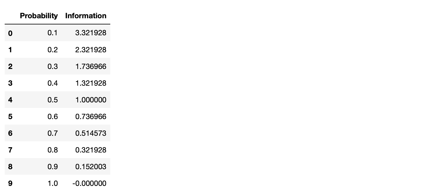
fig = px.line(df, x='Probability', y='Information', title='Probability vs Information')
fig.show()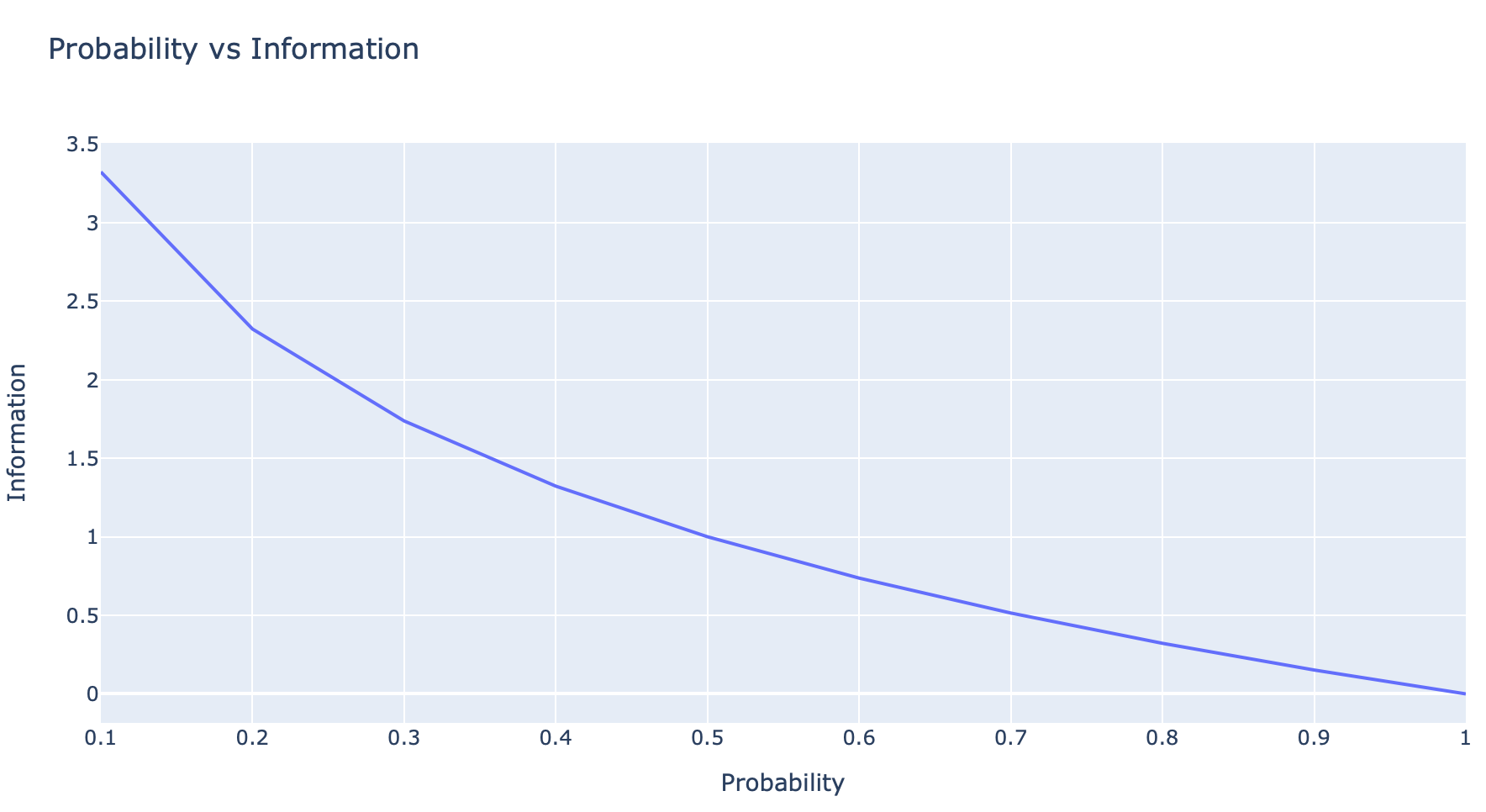
เราสามารถนำ Information Theory ไปประยุกต์ใช้ในการบีบอัดข้อมูลเพื่อประหยัดค่าใช้จ่ายในการสื่อสาร โดยสมมติว่าถ้าเรามีตัวอักษรอยู่ 4 ตัว ได้แก่ 'A', 'B', 'C' และ 'D' ซึ่งแต่ละตัวมีโอกาสปรากฏอยู่ในข้อความ (Text) ด้วยความน่าจะเป็น p เท่ากับ 1/2, 1/4, 1/8, และ 1/8 ตามลำดับ (รวมกันเท่ากับ 1.0) ดังนั้นเพื่อจะประหยัดจำนวน bit ในการส่งข้อมูล เราจะเข้ารหัสตัวอักษรทั้ง 4 ตัว ดังต่อไปนี้
'A' แทนด้วย 0 (1 bit)
'B' แทนด้วย 10 (2 bit)
'C' แทนด้วย 110 (3 bit)
'D' แทนด้วย 111 (3 bit)
Entropy
ดังนั้น เราสามารถคำนวณหาจำนวน bit โดยเฉลี่ยที่จำเป็นในการส่งข้อมูล สำหรับตัวอักษร 4 ตัว ที่มีการแจกแจงความน่าจะเป็น (Probability Distribution) เท่ากับ 1/2, 1/4, 1/8, และ 1/8 ได้ดังนี้
Average bit หรือ H(X) = (1/2 × 1) + (1/4 × 2) + (1/8 × 3) + (1/8 × 3) = 1.75เราเรียกจำนวน bit โดยเฉลี่ยดังกล่าวว่า Entropy (หรือ H(X) โดย X คือ Random Variable) ซึ่งคล้ายกับแนวคิดของ Entropy ในระบบทางกายภาพในวิชาฟิสิกส์ โดยทั้ง 2 จะให้ความสำคัญกับเรื่องของความไม่แน่นอน (Uncertainty)
สมมติว่ามีการโยนลูกเต๋า 1 ลูก ที่มีโอกาสออกแต่ละหน้าด้วยความน่าจะเป็น 1/6 (Uniform Probability Distribution) เราสามารถคาดหวังได้ว่าจำนวน bit โดยเฉลี่ย หรือ Entropy จะมีค่าดังนี้
P = [1/6, 1/6, 1/6, 1/6, 1/6, 1/6]

entropy = -sum([p * log2(p) for p in P])

print('entropy: %.3f bits' % entropy)
entropy: 2.585 bits
ในอีกแง่หนึ่ง Entropy นั้นบอกถึงความ Surprise โดยเฉลี่ย ซึ่งขึ้นอยู่กับลักษณะของการแจกแจงความน่าจะเป็น (Probability Distribution) ของเหตุการณ์หนึ่งๆ ดังตัวอย่างด้านล่าง
def entropy(events, ets=1e-15):
    return -sum([p * log2(p + ets) for p in events])

probs = [0.0, 0.1, 0.2, 0.3, 0.4, 0.5]

dists = [[p, 1.0 - p] for p in probs]

ents = [entropy(d) for d in dists]
df = pd.DataFrame(list(zip(probs, ents)), columns =['Probability Distribution', 'Entropy (bits)'])fig = px.line(df, x='Probability Distribution', y='Entropy (bits)', title='Probability Distribution vs Entropy')
fig.update_xaxes(ticktext=[str(d) for d in dists], tickvals = probs)
ซึ่งจากกราฟจะเห็นว่ายิ่งมีการกระจายตัวของความน่าจะเป็นที่สมดุล (Balanced Probability Distribution) ตามแกน x มากขึ้นเท่าไหร่ ความ Surprise หรือ Entropy ก็จะยิ่งมากขึ้นเท่านั้น
ยกตัวอย่างเช่น ในการโยนเหรียญที่มีโอกาสออกหัว 0% และออกก้อย 100% (Skewed Probability Distribution) ซึ่งไม่ว่าจะโยนกี่ครั้งมันก็จะออกก้อยตลอด ดังนั้นความ Surprise หรือ Entropy จึงเท่ากับ 0 ในขณะที่อีกกรณีหนึ่ง ถ้าในการโยนเหรียญมีโอกาสออกหัว 50% และออกก้อย 50% เท่ากัน (Balanced Probability Distribution) ความ Surprise หรือ Entropy จะมีค่าสูงสุดเท่ากับ 1 ครับ
Cross-Entropy
ทีนี้สมมติว่าในเวลาต่อมา การแจกแจงความน่าจะเป็น (Probability Distribution) ของตัวอักษร 4 ตัว ได้แก่ 'A', 'B', 'C' และ 'D' เปลี่ยนไปจากแบบ p = [1/2, 1/4, 1/8, 1/8] เป็นแบบ q = [1/8, 1/4, 1/2, 1/8]
events = ['A', 'B', 'C', 'D']
p = [1/2, 1/4, 1/8, 1/8]
q = [1/8, 1/4, 1/2, 1/8]
fig = go.Figure(data=[
go.Bar(name='Probability Distribution เก่า (p)', x=events, y=p, text=p, textposition='auto'),
go.Bar(name='Probability Distribution ใหม่ (q)', x=events, y=q, text=q, textposition='auto')
])
fig.update_layout(barmode='group')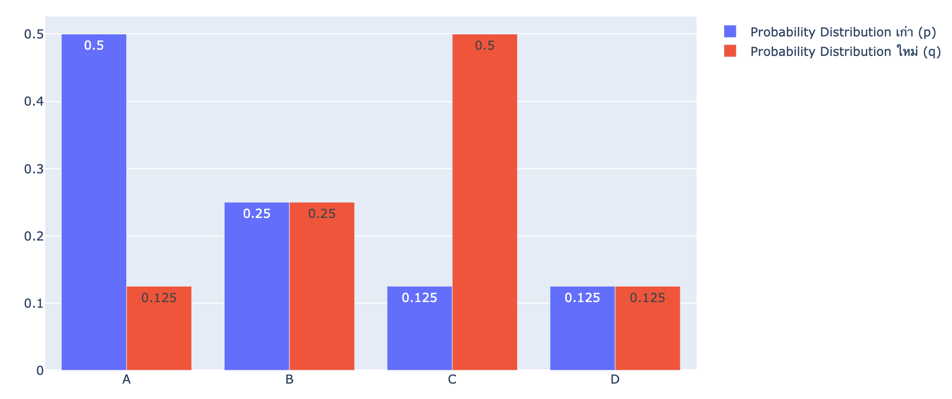
หากยังมีการเข้ารหัสตัวอักษรทั้ง 4 ตัว แบบเดิม จำนวน bit โดยเฉลี่ย ที่จำเป็นในการส่งข้อมูลจะเพิ่มขึ้นจาก 1.75 bit เป็น 2.5 bit!
Average bit หรือ H(p,q) = (1/2 × 3) + (1/4 × 2) + (1/8 × 1) + (1/8 × 3) = 2.5เราเรียกจำนวน bit โดยเฉลี่ย เมื่อมีการเข้ารหัสตัวอักษรแบบเดิม (p) ด้วยการแจกแจงความน่าจะเป็นใหม่ (q) นี้ว่า Cross-Entropy
def cross_entropy(p, q):
    return -sum([p[i]*log2(q[i]) for i in range(len(p))])
ce = cross_entropy(p, q)
print('H(P, Q): %.3f bits' % ce)H(P, Q): 2.500 bits
Cross-Entropy ถูกใช้ในการประมาณ Error ของ Classification Model ที่เกิดจากการแจกแจงความน่าจะเป็น 2 แบบ คือ ระหว่าง p กับ q ซึ่ง q คือ การแจกแจงความน่าจะเป็นที่โมเดลทำนาย [1/8, 1/4, 1/2, 1/8] และ p คือ การแจกแจงความน่าจะเป็นจริง [1/2, 1/4, 1/8, 1/8]
*H(P, Q) != H(Q, P)
Binary Classification Loss Functions
Binary Classification เป็น Model ที่มีการกำหนด Label หรือ Class เพียง 2 Class คือ ไม่เป็น Class 0 ก็เป็น Class 1 โดย ผลลัพธ์จากการทำนายของ Model จะบอกค่าความน่าจะเป็นว่ามีโอกาสที่จะเป็น Class 1 กี่เปอร์เซ็นต์
เราจะทดลอง Train Binary Classification Model โดยใช้ Binary Crossentropy Loss ของ Keras Framework ด้วย Dataset ที่ Make ขึ้นจากฟังก์ชัน make_circles ของ sklearn Library
*เพื่อจะทำให้ Model ทำนายผลออกมาเป็นค่าความน่าจะเป็น [0, 1] ว่ามีโอกาสที่จะเป็น Class 1 กี่เปอร์เซ็นต์ เราจะต้องคอนฟิก Activate Function ใน Output Layer แบบ Sigmoid
def sigmoid(x):
    return 1.0/(1+ np.exp(-x))

data = 25
result = sigmoid(data)

print(result)
0.999999999986112
Binary Crossentropy Loss
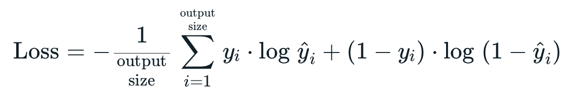
events = ['Class 0', 'Class 1']
actual = [1, 0, 1, 1, 0]
predicted = [0.7, 0.45, 0.9, 0.5, 0.3]

index = 0
p = [1-actual[index], actual[index]]
q = [1-predicted[index], predicted[index]]
fig = go.Figure(data=[
go.Bar(name='Actual Probability Distribution', x=events, y=p, text=p, textposition='auto'),
go.Bar(name='Predicted Probability Distribution', x=events, y=q, text=list(np.round(q,2)), textposition='auto')
])
fig.update_layout(barmode='group', title='Record 1')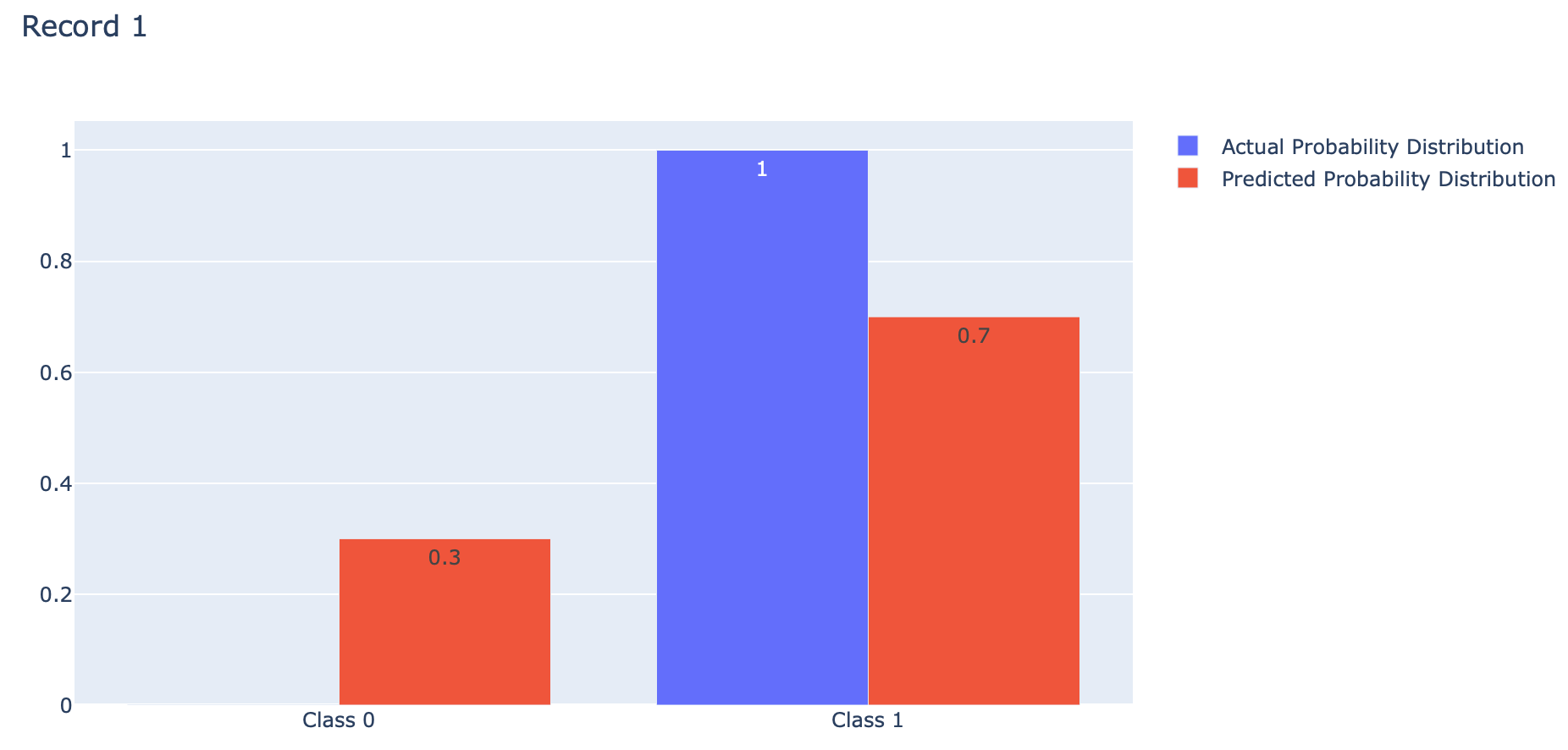
index = 1
p = [1-actual[index], actual[index]]
q = [1-predicted[index], predicted[index]]
fig = go.Figure(data=[
go.Bar(name='Actual Probability Distribution', x=events, y=p, text=p, textposition='auto'),
go.Bar(name='Predicted Probability Distribution', x=events, y=q, text=q, textposition='auto')
])
fig.update_layout(barmode='group', title='Record 2')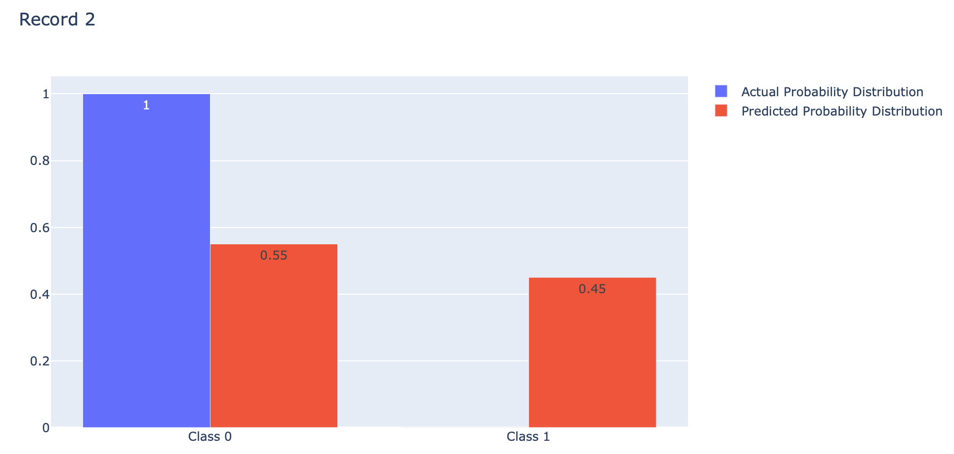
index = 2
p = [1-actual[index], actual[index]]
q = [1-predicted[index], predicted[index]]fig = go.Figure(data=[
go.Bar(name='Actual Probability Distribution', x=events, y=p, text=p, textposition='auto'),
go.Bar(name='Predicted Probability Distribution', x=events, y=q, text=np.round(q,2), textposition='auto')
])
fig.update_layout(barmode='group', title='Record 3')
index = 3
p = [1-actual[index], actual[index]]
q = [1-predicted[index], predicted[index]]fig = go.Figure(data=[
go.Bar(name='Actual Probability Distribution', x=events, y=p, text=p, textposition='auto'),
go.Bar(name='Predicted Probability Distribution', x=events, y=q, text=q, textposition='auto')
])
fig.update_layout(barmode='group', title='Record 4')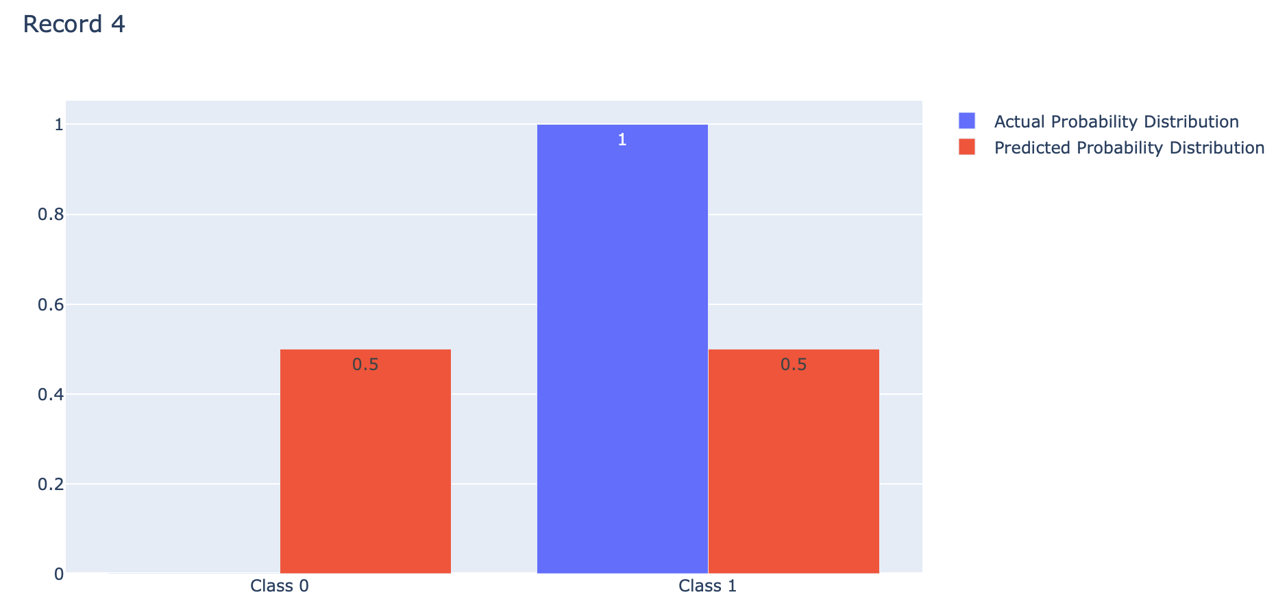
index = 4
p = [1-actual[index], actual[index]]
q = [1-predicted[index], predicted[index]]fig = go.Figure(data=[
go.Bar(name='Actual Probability Distribution', x=events, y=p, text=p, textposition='auto'),
go.Bar(name='Predicted Probability Distribution', x=events, y=q, text=q, textposition='auto')
])
fig.update_layout(barmode='group', title='Record 5')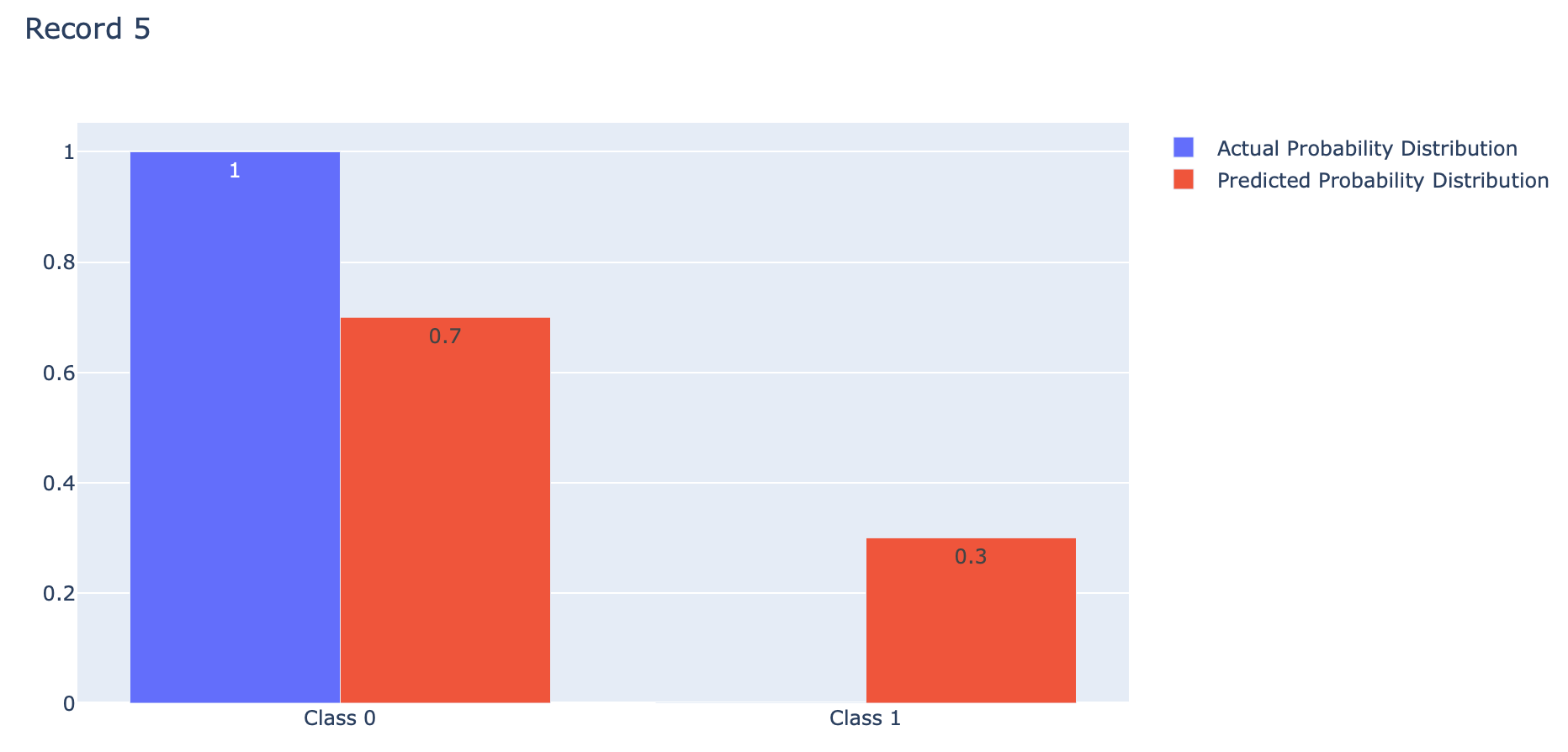
Binary Crossentropy คือ ค่าเฉลี่ยของ Cross-Entropy ที่เกิดจากการแจกแจงความน่าจะเป็น 2 แบบ คือ การแจกแจงความน่าจะเป็นที่เราอยากได้ (Actual) กับการแจกแจงความน่าจะเป็นที่ถูกประมาณโดย Model (Predicted) ของ Class 0 และ Class 1 ดังภาพด้านบน ซึ่งการได้ค่าเฉลี่ยน้อยนั้นดีกว่าการได้ค่าเฉลี่ยมาก โดย Binary Crossentropy Loss จะให้ค่าเฉลี่ยต่ำสุดคือ 0
อย่างไรก็ตาม Binary Crossentropy Loss ของ Keras จะมีการใช้งาน Logarithm ฐาน e แทนที่จะเป็น Logarithm ฐาน 2 เหมือนกับตัวอย่างที่ผ่านมาครับ
def binary_cross_entropy_loss(actual, predicted):
sum = 0
for i in range(len(actual)):
sum=sum+actual[i]*log(predicted[i])+(1-actual[i])*log(1-predicted[i])
return -sum/len(actual)
binary_cross_entropy_loss(actual, predicted)0.4219389169701714
loss = tf.keras.losses.binary_crossentropy(actual, predicted)
loss.numpy()0.42193872
actual = [1, 0, 1, 1, 0]
predicted = [1.0, 0.0, 1.0, 1.0, 0.0]
loss = tf.keras.losses.binary_crossentropy(actual, predicted)
loss.numpy()0.0
Example
เราจะทดลอง Train Model แบบ Binary Classification จากข้อมูลที่ Make ขึ้นมาด้วยฟังก์ชัน make_circles ตามขั้นตอนต่อไปนี้
- Import Library ที่จำเป็นต้องใช้ในการทดลอง
to_categorical = tf.keras.utils.to_categorical
from tensorflow.keras.utils import to_categorical
import plotly
import plotly.graph_objs as go
import plotly.express as px
from sklearn.datasets import make_circles
from sklearn.datasets import make_blobs
from sklearn.model_selection import train_test_split
import pandas as pd- สร้าง Dataset แบบ 2 Class โดยใช้ Function make_circles ของ Sklearn
x, y = make_circles(n_samples=5000, noise=0.1, random_state=1)- แบ่งข้อมูลสำหรับ Train และ Test โดยการสุ่มในสัดส่วน 50:50
x_train, x_val, y_train, y_val = train_test_split(x, y, test_size=0.4, shuffle= True)
x_train.shape, x_val.shape, y_train.shape, y_val.shape((3000, 2), (2000, 2), (3000,), (2000,))
- นำ Dataset ส่วนที่ Train มาแปลงเป็น DataFrame โดยเปลี่ยนชนิดข้อมูลใน Column "class" เป็น String เพื่อทำให้สามารถแสดงสีแบบไม่ต่อเนื่องได้ แล้วนำไป Plot
x_train_pd = pd.DataFrame(x_train, columns=['x', 'y'])
y_train_pd = pd.DataFrame(y_train, columns=['class'], dtype='str')
df = pd.concat([x_train_pd, y_train_pd], axis=1)fig = px.scatter(df, x="x", y="y", color="class")
fig.show()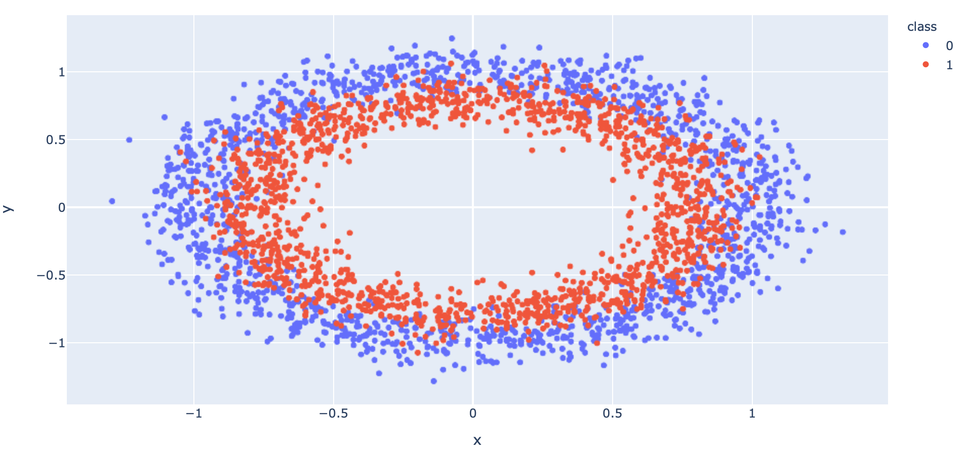
- นิยาม Model โดยกำหนด Activation Function ใน Layer สุดท้ายเป็น sigmoid
model = tf.keras.models.Sequential()
model.add(tf.keras.layers.Dense(60, input_dim=2, activation='relu', kernel_initializer='he_uniform'))
model.add(tf.keras.layers.Dropout(0.2))
model.add(tf.keras.layers.Dense(1, activation='sigmoid'))- Compile Model โดยกำหนด Loss Function เป็น binary_crossentropy
opt = tf.keras.optimizers.SGD(learning_rate=0.01, momentum=0.9)
model.compile(loss='binary_crossentropy', optimizer=opt, metrics=['accuracy'])- Train Model
his = model.fit(x_train, y_train, validation_data=(x_val, y_val), epochs=2000, verbose=1, batch_size = 256)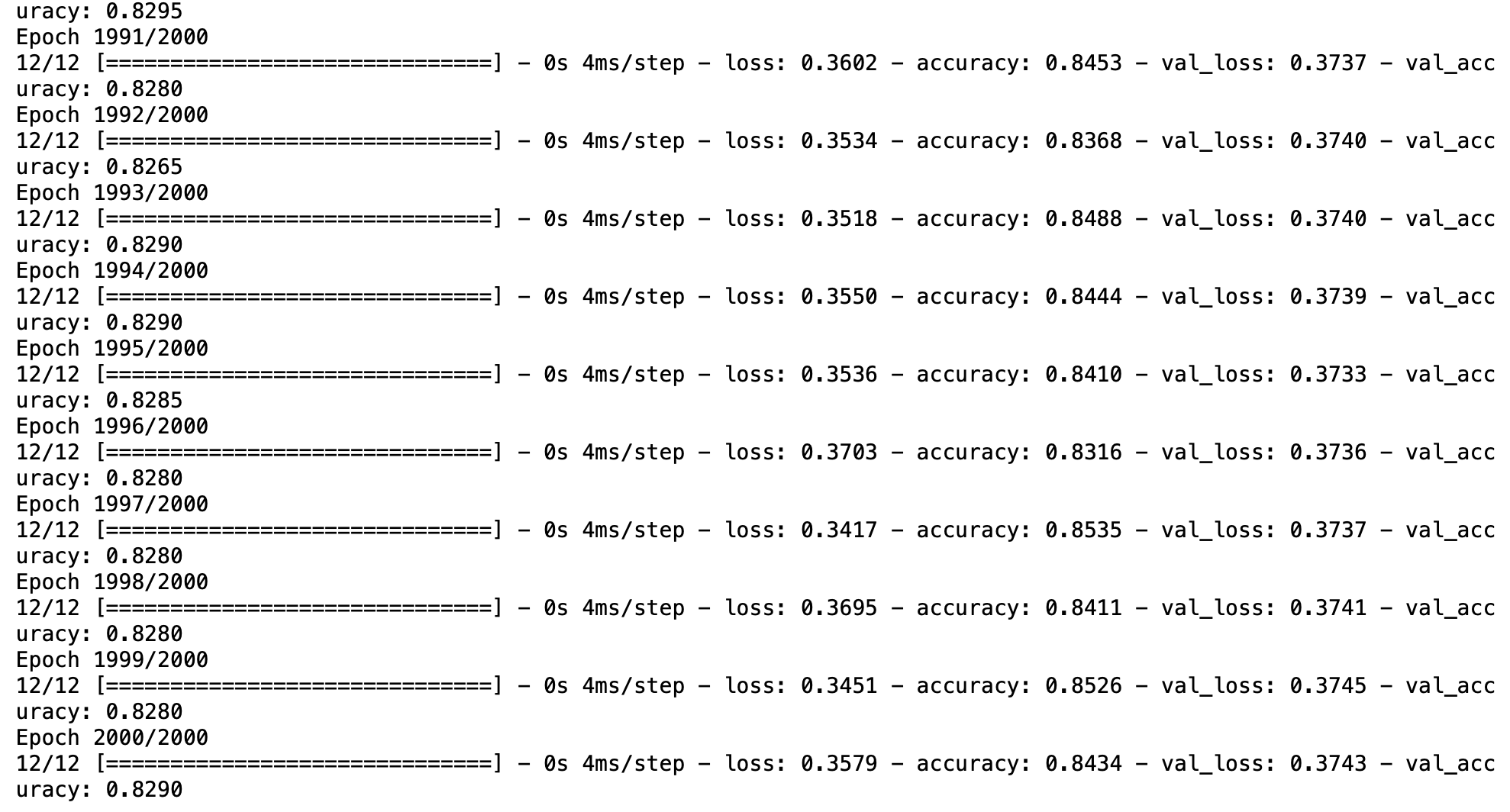
- Plot Loss
h1 = go.Scatter(y=his.history['loss'],
mode="lines",
line=dict(
width=2,
color='blue'),
name="loss"
)
h2 = go.Scatter(y=his.history['val_loss'],
mode="lines",
line=dict(
width=2,
color='red'),
name="val_loss"
)
data = [h1,h2]
layout1 = go.Layout(title='Loss',
xaxis=dict(title='epochs'),
yaxis=dict(title=''))
fig1 = go.Figure(data = data, layout=layout1)
plotly.offline.iplot(fig1)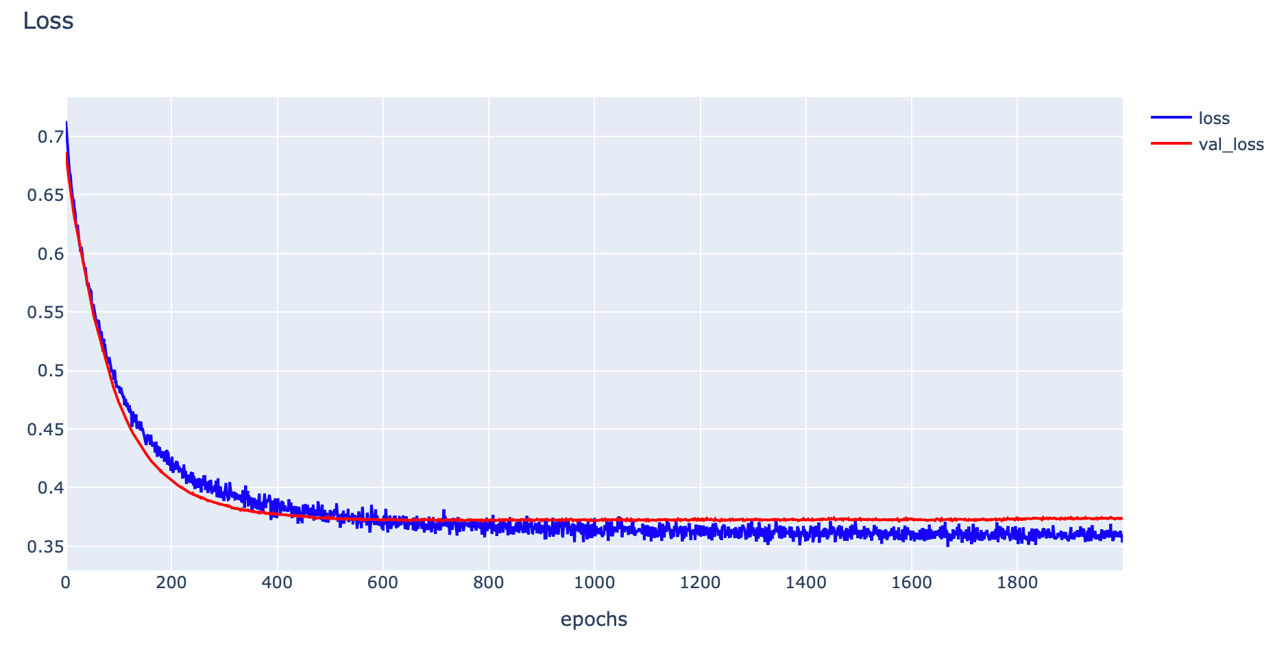
- Plot Accuracy
h1 = go.Scatter(y=his.history['accuracy'],
mode="lines", line=dict(
width=2,
color='blue'),
name="acc"
)
h2 = go.Scatter(y=his.history['val_accuracy'],
mode="lines", line=dict(
width=2,
color='red'),
name="val_acc"
)
data = [h1,h2]
layout1 = go.Layout(title='Accuracy',
xaxis=dict(title='epochs'),
yaxis=dict(title=''))
fig1 = go.Figure(data = data, layout=layout1)
plotly.offline.iplot(fig1)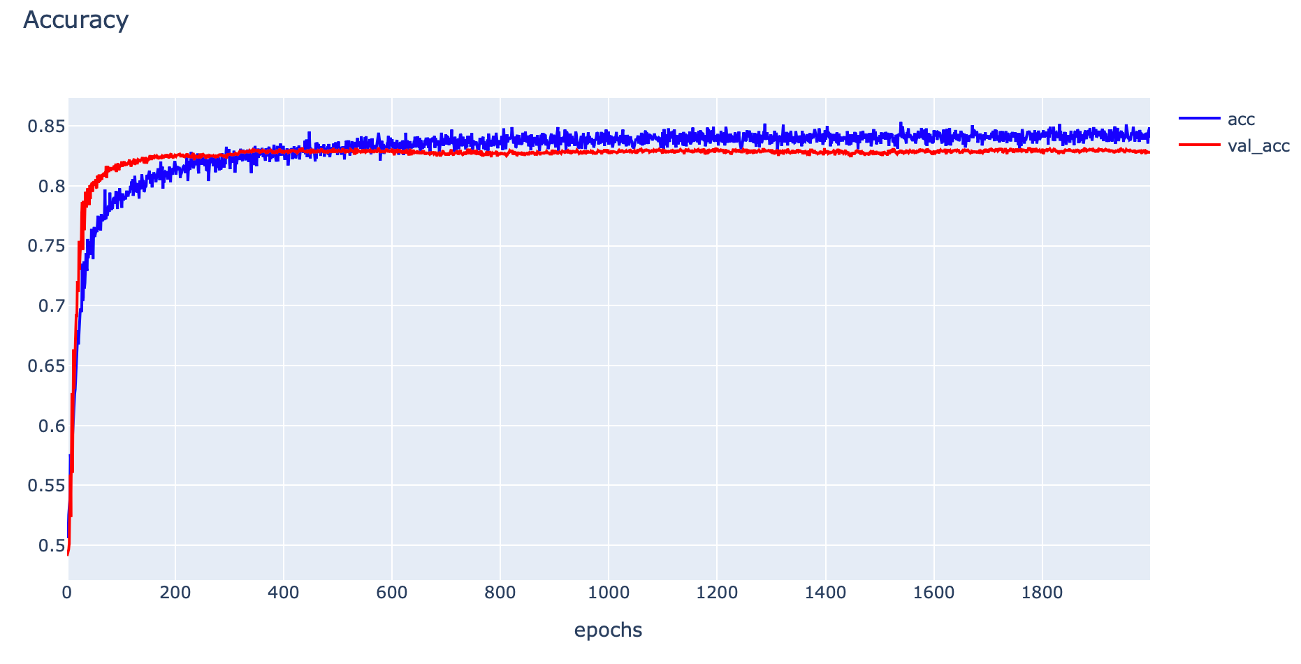
- Evaluate Model
_, train_acc = model.evaluate(x_train, y_train, verbose=0)
_, val_acc = model.evaluate(x_val, y_val, verbose=0)
print('Train: %.4f, Validation: %.4f' % (train_acc, val_acc))Train: 0.8543, Validation: 0.8290
res = model.predict(x_train)
print(res[:10])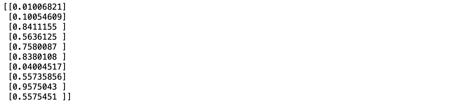
จากภาพด้านบน Model จะส่งผลการทำนายเป็นค่าความน่าจะเป็นว่ามีโอกาสที่จะเป็น Class 1 กี่เปอร์เซ็นต์ ซึ่งโดย Default จะทำนายว่าเป็น Class 1 เมื่อค่าความน่าจะเป็นมากกว่า 0.5
Multi-Class Classification Loss Functions
Multi-Class Classification เป็น Model ที่มีการกำหนด Label หรือ Class มากกว่า 2 Class ซึ่งโดยมากจะเริ่มต้นที่ Class 0 จนถึง num_class - 1 ผลลัพธ์ของ Model จะบอกถึงค่าความเชื่อมั่นในการทำนายของแต่ละ Class โดยค่าความเชื่อมั่นทุก Class รวมกันจะเท่ากับ 1.0
เราจะทดลอง Train Multi-Class Classification Model โดยใช้ Categorical Crossentropy Loss ของ Keras Framework ด้วย Dataset ที่ Make ขึ้นจากฟังก์ชัน make_blobs ของ sklearn Library
*เพื่อจะทำให้ Model ทำนายผลออกมาเป็นค่าความเชื่อมั่นที่ทุก Class รวมกันเท่ากับ 1.0 เราจะต้องคอนฟิก Activate Function ใน Output Layer แบบ Softmax ครับ
def softmax(vector):
e = np.exp(vector)
return e/e.sum()
data = [1, 3, 2.5]
result = softmax(data)
print(result)
print(sum(result))[0.07769558 0.57409699 0.34820743]
1.0
Categorical Crossentropy Loss

events = ['Class 0', 'Class 1', 'Class 2']
actual = [[1, 0, 0], [0, 1, 0], [0, 0, 1]]
predicted = [[0.9, 0.05, 0.05], [0.05, 0.89, 0.06], [0.05, 0.01, 0.94]]
p = actual[0]
q = predicted[0]fig = go.Figure(data=[
go.Bar(name='Actual Probability Distribution', x=events, y=p, text=p, textposition='auto'),
go.Bar(name='Predicted Probability Distribution', x=events, y=q, text=q, textposition='auto')
])
fig.update_layout(barmode='group', title='Record 1')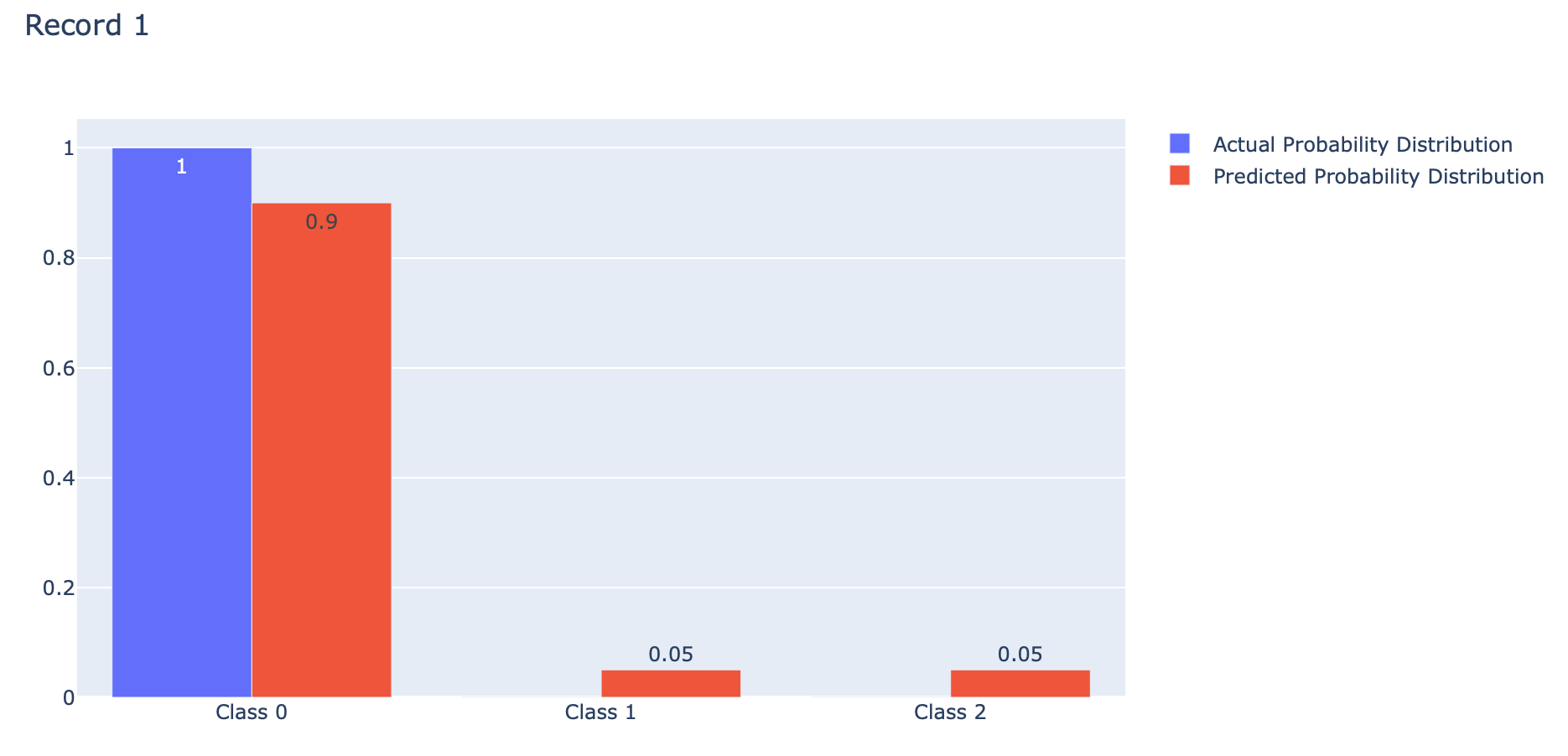
p = actual[1]
q = predicted[1]
fig = go.Figure(data=[
    go.Bar(name='Actual Probability Distribution', x=events, y=p, text=p, textposition='auto'),
    go.Bar(name='Predicted Probability Distribution', x=events, y=q, text=q, textposition='auto')
])

fig.update_layout(barmode='group', title='Record 2')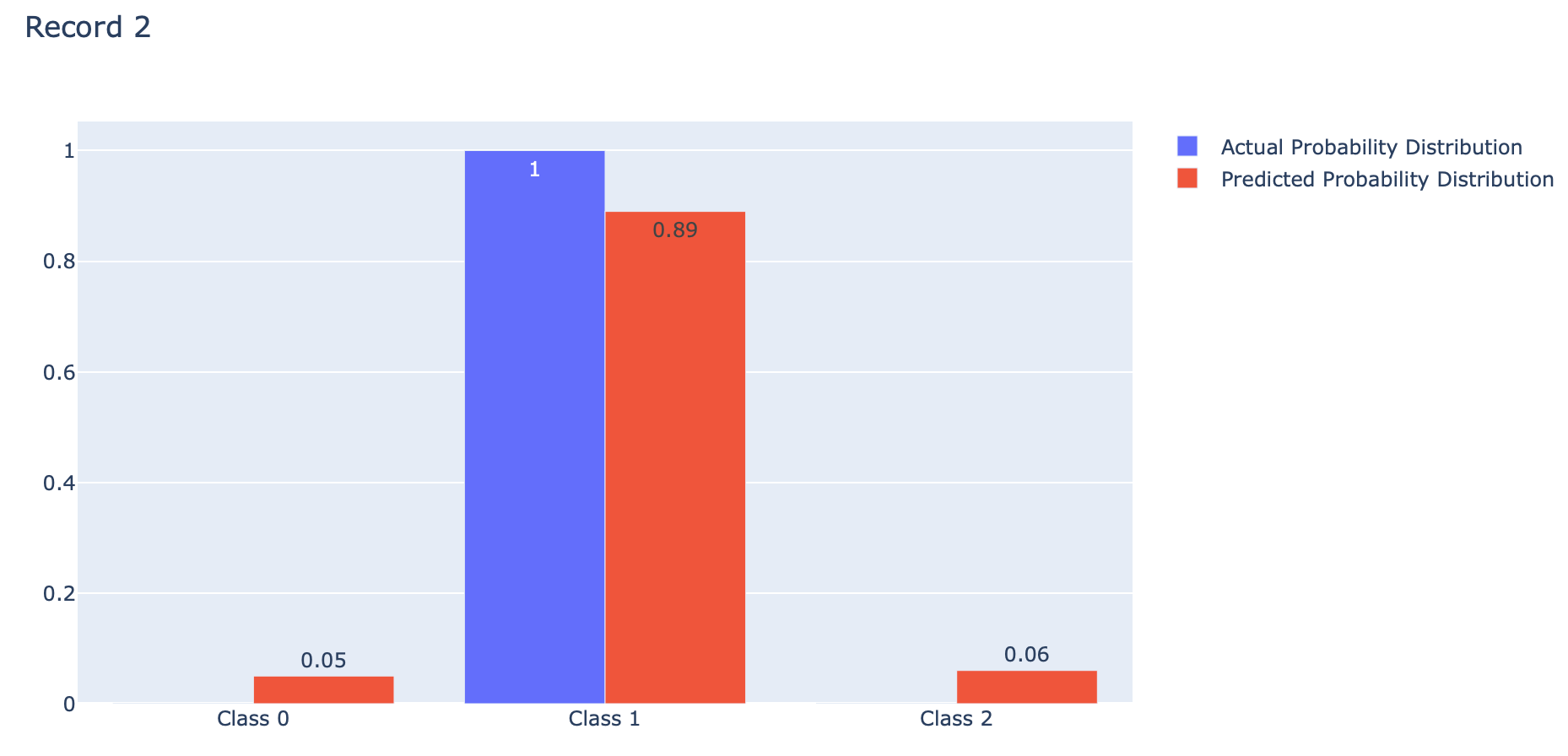
p = actual[2]
q = predicted[2]
fig = go.Figure(data=[
go.Bar(name='Actual Probability Distribution', x=events, y=p, text=p, textposition='auto'),
go.Bar(name='Predicted Probability Distribution', x=events, y=q, text=q, textposition='auto')
])
fig.update_layout(barmode='group', title='Record 3')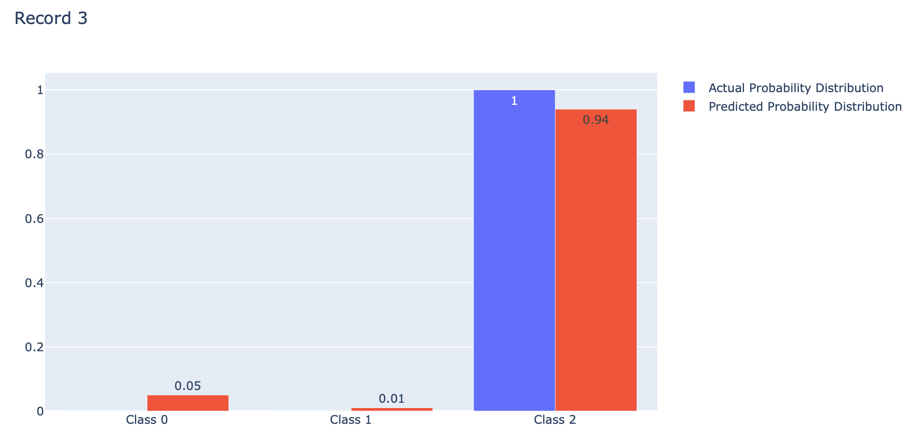
Categorical Crossentropy คือ ค่าเฉลี่ยของ Cross-Entropy ที่เกิดจากการแจกแจงความน่าจะเป็น 2 แบบ คือ การแจกแจงความน่าจะเป็นที่เราอยากได้ (Actual) กับการแจกแจงความน่าจะเป็นที่ถูกประมาณโดย Model (Predicted) ของ Class ต่างๆ (Class 0, 1, 2) ดังภาพด้านบน ซึ่งการได้ค่าเฉลี่ยน้อยนั้นดีกว่าการได้ค่าเฉลี่ยมาก โดย Categorical Crossentropy Loss ของ Keras จะมีการใช้งาน Logarithm ฐาน e เช่นเดียวกับ Binary Crossentropy Loss ครับ
def categorical_cross_entropy(actual, predicted):
sum = 0.0
for i in range(len(actual)):
for j in range(len(actual[i])):
sum += actual[i][j] * log(1e-15 + predicted[i][j])
mean = 1.0 / len(actual) * sum
return -mean
np.around(categorical_cross_entropy(actual, predicted),5)0.09459
*บวกตัวเลขขนาดเล็ก (1e+15) เพื่อป้องกันการคำนวนค่า log ของ 0
cce = tf.keras.losses.CategoricalCrossentropy()
np.around(cce(actual, predicted).numpy(),5)0.09459
Example
เราจะทดลอง Train Model แบบ Multi-Class Classification จากข้อมูลที่ Make ขึ้นมาด้วยฟังก์ชัน make_blobs ตามขั้นตอนต่อไปนี้
- สร้าง Dataset แบบ 3 Class โดยใช้ Function make_blobs ของ Sklearn
x, y = make_blobs(n_samples=1000, centers=3, n_features=2, cluster_std=2, random_state=2)- เข้ารหัสผลเฉลยแบบ One-hot Encoding เพื่อสร้างการแจกแจงความน่าจะเป็นที่เราอยากได้ (Actual Probability Distribution)
y = to_categorical(y)
y[:10]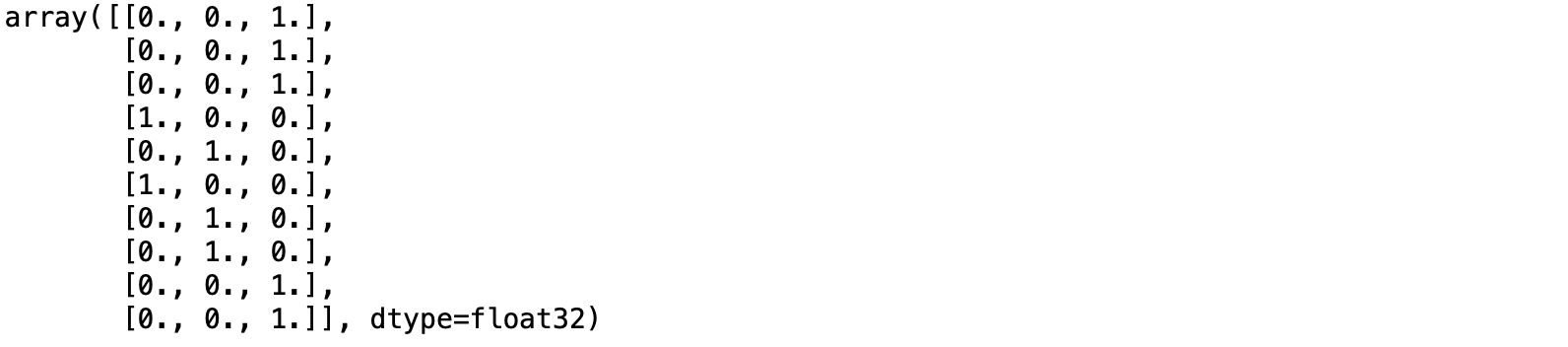
- แบ่งข้อมูลสำหรับ Train และ Test โดยการสุ่มในสัดส่วน 50:50
x_train, x_val, y_train, y_val = train_test_split(x, y, test_size=0.5, shuffle= True)
x_train.shape, x_val.shape, y_train.shape, y_val.shape((500, 2), (500, 2), (500, 3), (500, 3))
- นำ Dataset ส่วนที่ Train มาแปลงเป็น DataFrame โดยเปลี่ยนชนิดข้อมูลใน Column "class" เป็น String เพื่อทำให้สามารถแสดงสีแบบไม่ต่อเนื่องได้ แล้วนำไป Plot
y = np.argmax(y_train,axis=1)
x_train_pd = pd.DataFrame(x_train, columns=['x', 'y'])
y_train_pd = pd.DataFrame(y, columns=['class'], dtype='str')
df = pd.concat([x_train_pd, y_train_pd], axis=1)fig = px.scatter(df, x="x", y="y", color="class")
fig.show()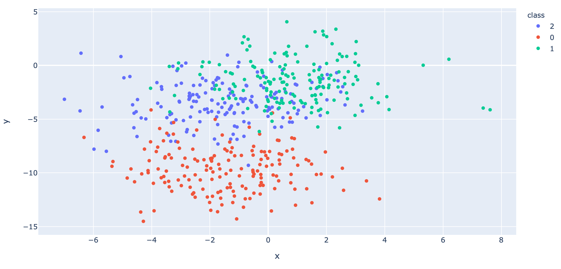
- นิยาม Model แบบ 3 Class โดยกำหนด Activation Function ใน Layer สุดท้ายเป็น softmax
model = tf.keras.models.Sequential()
model.add(tf.keras.layers.Dense(60, input_dim=2, activation='relu', kernel_initializer='he_uniform'))
model.add(tf.keras.layers.Dropout(0.2))
model.add(tf.keras.layers.Dense(3, activation='softmax'))- Compile Model โดยกำหนด Loss Function เป็น categorical_crossentropy
opt = tf.keras.optimizers.SGD(learning_rate=0.01, momentum=0.9)
model.compile(loss='categorical_crossentropy', optimizer=opt, metrics=['accuracy'])- Train Model
his = model.fit(x_train, y_train, validation_data=(x_val, y_val), epochs=1000, verbose=1, batch_size = 128)
- Plot Loss
h1 = go.Scatter(y=his.history['loss'],
mode="lines",
line=dict(
width=2,
color='blue'),
name="loss"
)
h2 = go.Scatter(y=his.history['val_loss'],
mode="lines",
line=dict(
width=2,
color='red'),
name="val_loss"
)
data = [h1,h2]
layout1 = go.Layout(title='Loss',
xaxis=dict(title='epochs'),
yaxis=dict(title=''))
fig1 = go.Figure(data = data, layout=layout1)
plotly.offline.iplot(fig1)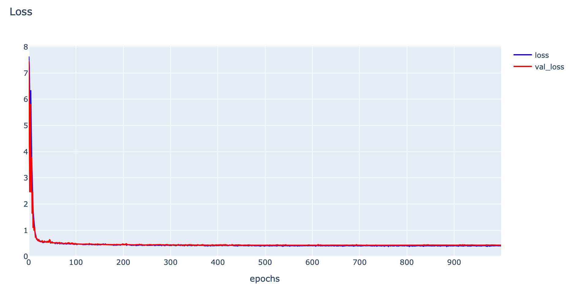
- Plot Accuracy
h1 = go.Scatter(y=his.history['accuracy'],
mode="lines",
line=dict(
width=2,
color='blue'),
name="acc"
)
h2 = go.Scatter(y=his.history['val_accuracy'],
mode="lines",
line=dict(
width=2,
color='red'),
name="val_acc"
)
data = [h1,h2]
layout1 = go.Layout(title='Accuracy',
xaxis=dict(title='epochs'),
yaxis=dict(title=''))
fig1 = go.Figure(data = data, layout=layout1)
plotly.offline.iplot(fig1)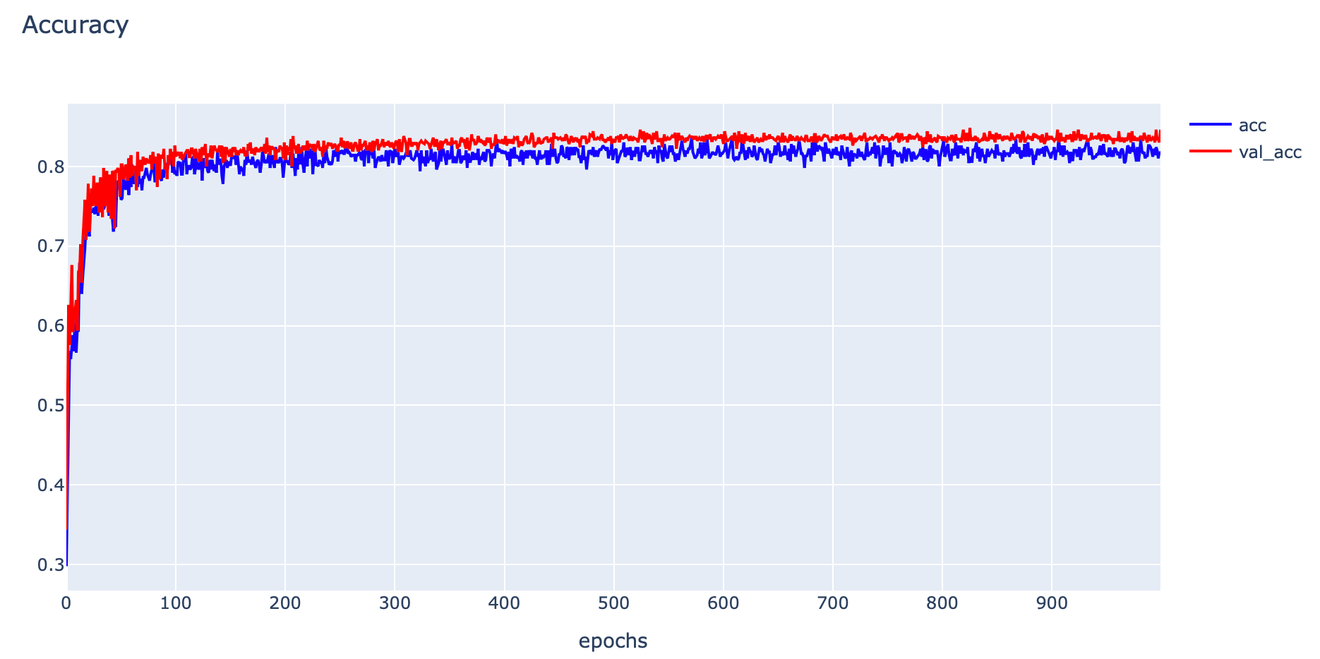
- Evaluate Model
_, train_acc = model.evaluate(x_train, y_train, verbose=0)
_, val_acc = model.evaluate(x_val, y_val, verbose=0)
print('Train: %.4f, Validation: %.4f' % (train_acc, val_acc))Train: 0.8260, Validation: 0.8460
res = model.predict(x_train)
print(np.round(res[:10],3))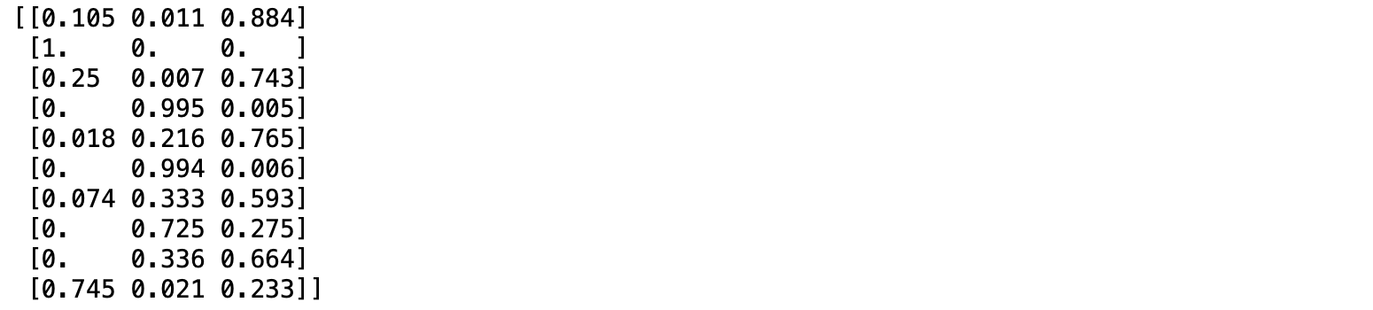
จากภาพด้านบน แสดงค่าความเชื่อมั่นในการทำนายของแต่ละ Class (Class 0, 1, 2) จาก Input Data 10 Record โดยค่าความเชื่อมั่นทุก Class รวมกันเท่ากับ 1.0
Sparse Categorical Crossentropy Loss
โดย Default แล้ว ในการสร้าง Model แบบ Multi-Class Classification เราจะคอนฟิก Loss Function เป็น Categorical Crossentropy Loss แต่สำหรับปัญหาบางปัญหาที่มีผลเฉลย (Label) จำนวนมากๆ การเข้ารหัสผลเฉลยแบบ One-hot Encoding เพื่อสร้างการแจกแจงความน่าจะเป็นแบบที่เราอยากได้ (Actual Probability Distribution) จะทำให้สิ้นเปลือง Memory
Sparse Categorical Crossentropy สามารถแก้ปัญหานี้ได้โดยไม่ต้องสร้างผลเฉลยแบบ One-hot Encoding แต่ยังคงมีการคำนวนค่า Cross-entropy ได้เหมือนเดิม ซึ่งในการคอนฟิก Model ให้ใช้งาน Sparse Categorical Crossentropy Loss เรายังคงใช้ Activate Function เป็น Softmax ที่ Output Layer เช่นเดิม
Example
เราจะทดลอง Train Model แบบ Multi-Class Classification จากข้อมูลที่ Make ขึ้นมาด้วยฟังก์ชัน make_blobs ตามขั้นตอนต่อไปนี้
- สร้าง Dataset แบบ 20 Class โดยใช้ Function make_blobs ของ Sklearn
x, y = make_blobs(n_samples=10000, centers=20, n_features=2, cluster_std=0.1, random_state=2)- แบ่งข้อมูลสำหรับ Train และ Test โดยการสุ่มในสัดส่วน 50:50
x_train, x_val, y_train, y_val = train_test_split(x, y, test_size=0.5, shuffle= True)
x_train.shape, x_val.shape, y_train.shape, y_val.shape((5000, 2), (5000, 2), (5000,), (5000,))
- นำ Dataset ส่วนที่ Train มาแปลงเป็น DataFrame โดยเปลี่ยนชนิดข้อมูลใน Column "class" เป็น String เพื่อทำให้สามารถแสดงสีแบบไม่ต่อเนื่องได้ แล้วนำไป Plot
x_train_pd = pd.DataFrame(x_train, columns=['x', 'y'])
y_train_pd = pd.DataFrame(y_train, columns=['class'], dtype='str')

df = pd.concat([x_train_pd, y_train_pd], axis=1)
fig = px.scatter(df, x="x", y="y", color="class")
fig.show()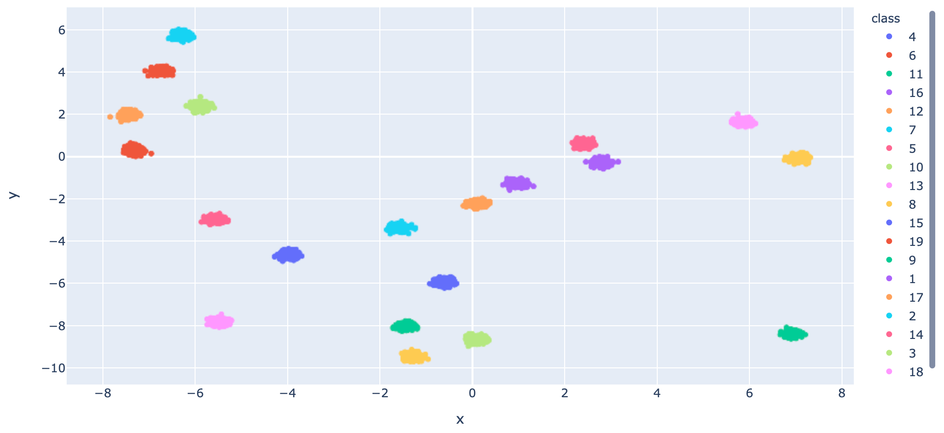
- นิยาม Model แบบ 20 Class โดยกำหนด Activation Function ใน Layer สุดท้ายเป็น softmax
model = tf.keras.models.Sequential()
model.add(tf.keras.layers.Dense(60, input_dim=2, activation='relu', kernel_initializer='he_uniform'))
model.add(tf.keras.layers.Dropout(0.2))
model.add(tf.keras.layers.Dense(20, activation='softmax'))- Compile Model โดยกำหนด Loss Function เป็น sparse_categorical_crossentropy
opt = tf.keras.optimizers.SGD(learning_rate=0.01, momentum=0.9)
model.compile(loss='sparse_categorical_crossentropy', optimizer=opt, metrics=['accuracy'])- Train Model
his = model.fit(x_train, y_train, validation_data=(x_val, y_val), epochs=1000, verbose=1, batch_size = 128)
- Plot Loss
h1 = go.Scatter(y=his.history['loss'],
                    mode="lines",
                    line=dict(
                        width=2,
                        color='blue'),
                        name="loss"
                   )
h2 = go.Scatter(y=his.history['val_loss'],
                    mode="lines",
                    line=dict(
                        width=2,
                        color='red'),
                        name="val_loss"
                   )

data = [h1,h2]
layout1 = go.Layout(title='Loss',
                   xaxis=dict(title='epochs'),
                   yaxis=dict(title=''))
fig1 = go.Figure(data = data, layout=layout1)
plotly.offline.iplot(fig1)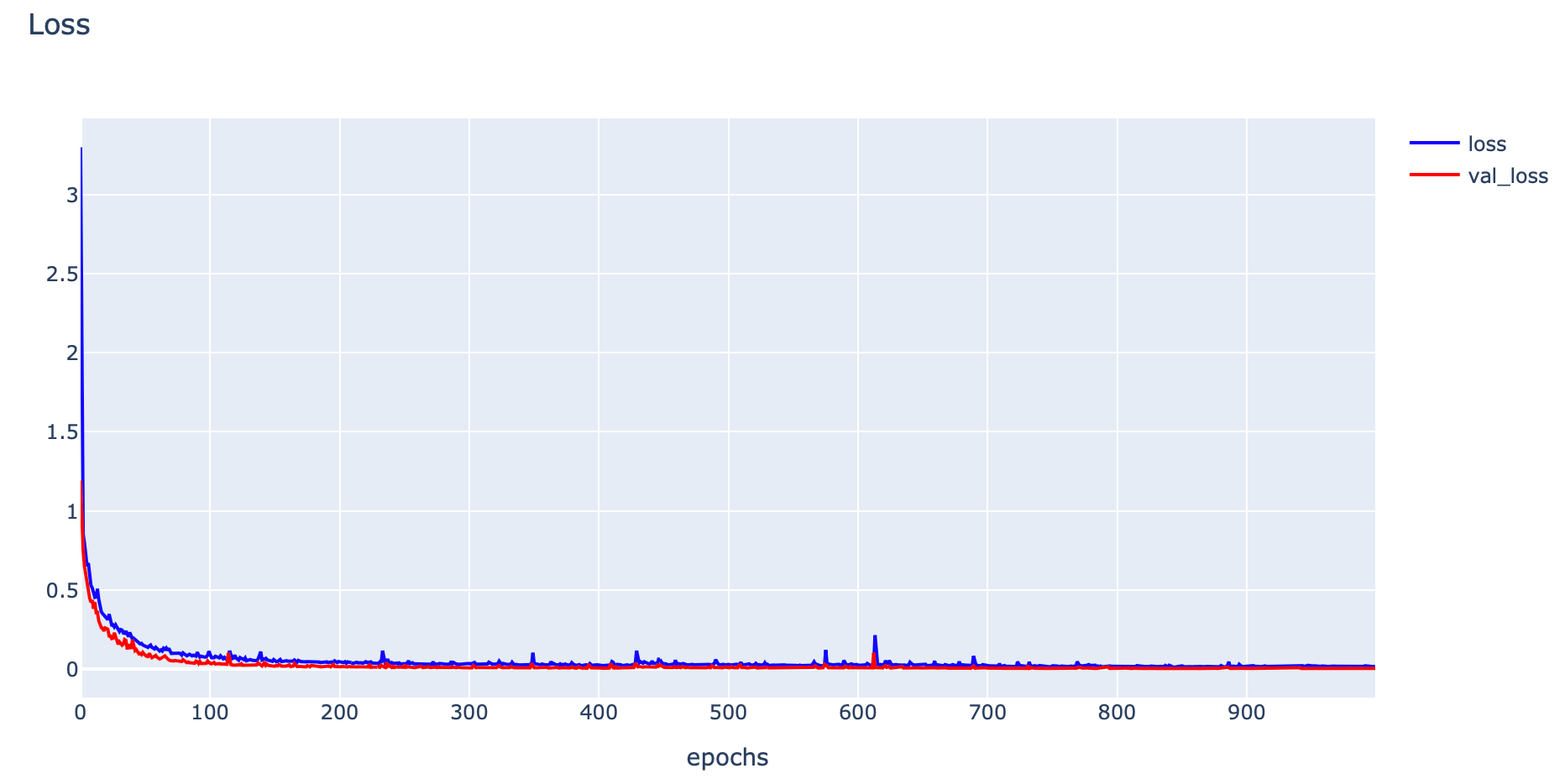
- Plot Accuracy
h1 = go.Scatter(y=his.history['accuracy'],
                    mode="lines", line=dict(
                    width=2,
                    color='blue'),
                    name="acc"
                   )
h2 = go.Scatter(y=his.history['val_accuracy'],
                    mode="lines", line=dict(
                    width=2,
                    color='red'),
                    name="val_acc"
                   )

data = [h1,h2]
layout1 = go.Layout(title='Accuracy',
                   xaxis=dict(title='epochs'),
                   yaxis=dict(title=''))
fig1 = go.Figure(data = data, layout=layout1)
plotly.offline.iplot(fig1)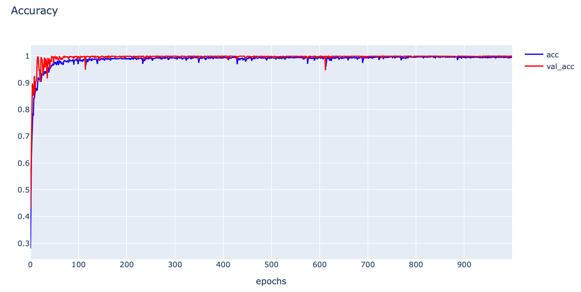
- Evaluate Model
_, train_acc = model.evaluate(x_train, y_train, verbose=0)
_, val_acc = model.evaluate(x_val, y_val, verbose=0)
print('Train: %.4f, Validation: %.4f' % (train_acc, val_acc))
Train: 0.9994, Validation: 0.9992
res = model.predict(x_train)

print(np.round(res[:1],3))
จากภาพด้านบน แสดงค่าความเชื่อมั่นในการทำนายของแต่ละ Class (Class 0 - 19) จาก Input Data 1 Record โดยค่าความเชื่อมั่นทุก Class รวมกันเท่ากับ 1.0
- การเลือกใช้ Loss Function ในการพัฒนา Deep Learning Model (ตอนที่ 1)
- การเลือกใช้ Loss Function ในการพัฒนา Deep Learning Model (ตอนที่ 2)