บทความโดย ผศ.ดร.ณัฐโชติ พรหมฤทธิ์
ภาควิชาคอมพิวเตอร์
คณะวิทยาศาสตร์
มหาวิทยาลัยศิลปากร

Deep Learning Model ที่ถูก Train ด้วย Stochastic Gradient Descent Optimization Algorithm มีกระบวนการทำงานหลักๆ 2 ส่วน ได้แก่ 1) Forward Propagation และ 2) Back-propagation โดยในการทำ Forward Propagation จะมีการประมาณ Error หรือ Loss ของ Model ด้วย Loss Function และในการทำ Back-propagation จะมีการปรับค่า Parameter (Weight และ Bias) จากการหาอนุพันธ์ของ Loss Function เพื่อให้ได้ค่า Loss ที่ลดลง โดยเป้าหมายหลักของ Optimization Algorithm คือ การทำให้ Loss เคลื่อนที่ไปยังจุดต่ำสุดบน Loss Surface (Global Minima)

ซึ่งการเลือกใช้ Loss Function ได้อย่างเหมาะสมกับปัญหา รวมทั้งการคอนฟิก Output Layer ของ Model ที่เหมาะสมกับ Loss Function ที่เลือก เป็นสิ่งสำคัญอย่างยิ่งในการ Train Deep Learning Model

ผมจะขอแบ่งบทความออกเป็น 2 ตอน เพื่อให้ผู้อ่านได้ทำ Workshop ที่มีการคอนฟิก Model แบบ Regression, Autoencoder และ Classification ด้วย Loss Function 6 ตัว ได้แก่

• Mean Squared Error Loss
• Mean Squared Logarithmic Error Loss
• Mean Absolute Error Loss
• Binary Crossentropy Loss (ตอนต่อไป)
• Categorical Crossentropy Loss (ตอนต่อไป)
• Sparse Categorical Crossentropy Loss (ตอนต่อไป)

Regression Loss Functions

Model แบบ Regression จะทำนายค่าโดยมีผลลัพธ์เป็นเลขจำนวนจริง ซึ่งในบทความนี้ เราจะทดลอง Train Regression Model โดยใช้ Loss Function 2 แบบ ได้แก่ 1) Mean Squared Error Loss และ 2) Mean Squared Logarithmic Error Loss โดย Loss Function ทั้ง 2 ตัว จะมีความเหมาะสมกับการแก้ปัญหาของ Model แตกต่างกัน

Mean Squared Error Loss

Mean Squared Error Loss เป็นตัวเลือกแรกในการแก้ปัญหาแบบ Regression ครับ โดย Mean Squared Error (MSE) คือ ค่าเฉลี่ยของผลต่างยกกำลังสอง ((y - ŷ)^2) ระหว่างค่าที่เป็นเลขจำนวนจริงที่เป็นผลเฉลย (y) กับค่าที่เกิดจากการทำนายของ Model (ŷ) ซึ่ง MSE จะไม่ติดลบ และจะมีค่าน้อยที่สุด คือ 0.0 เพราะผลต่างยกกำลังสองตามสมการด้านบน นอกจากนี้การยกกำลังสองของ MSE ยังจะทำให้ความผิดพลาดที่มีขนาดใหญ่มีผลต่อ Error ได้มากกว่าความผิดพลาดที่มีขนาดเล็ก หรือกล่าวได้อีกอย่างหนึ่งว่า Model ที่ใช้ Mean Squared Error Loss จะถูกลงโทษอย่างหนักเมื่อมันทำความผิดร้ายแรง

True value	Predicted value		MSE loss
10		20			100
1,000		2,000			1,000,000

Example

เราจะทดลอง Train Model แบบ Regression จากข้อมูลที่ Make ขึ้นมาด้วยฟังก์ชัน make_regression ของ Library Sklearn ตามขั้นตอนต่อไปนี้

• Import Library ที่จำเป็นต้องใช้ในการทดลอง

import tensorflow as tf
mnist = tf.keras.datasets.mnist

from sklearn.model_selection import train_test_split
from sklearn.manifold import TSNE
from sklearn.datasets import make_regression
from sklearn.preprocessing import StandardScaler
# from sklearn.datasets import load_boston

import pandas as pd

import plotly.express as px
import plotly
import plotly.graph_objs as go

import seaborn as sns
import matplotlib.pyplot as plt

import numpy as np

• สร้าง Dataset แบบ Regression ที่มี Input Feature เท่ากับ 10 (มิติ) จำนวน 3,000 Record ด้วยฟังก์ชัน make_regression

x, y = make_regression(n_samples=3000, n_features=10, noise=0.2, random_state=1)

x.shape, y.shape

((3000, 10), (3000,))

• ทำ Scaling Data แบบ Standardization (เนื่องจากเรารู้ว่าฟังก์ชัน make_regression จะ make Dataset แบบ Normal Distribution) เพื่อทำให้ Mean ของ Dataset เท่ากับ 0 และ Standard Deviation เท่ากับ 1

x = StandardScaler().fit_transform(x)
y = StandardScaler().fit_transform(y.reshape(len(y),1))[:,0]

* โดยปกติ Model จะมีประสิทธิภาพยิ่งขึ้นเมื่อมีการทำ Scaling กับ Input Data และ Output Data

• แบ่งข้อมูลสำหรับ Train และ Test โดยการสุ่มในสัดส่วน 50:50

x_train, x_val, y_train, y_val = train_test_split(x, y, test_size=0.5, shuffle= True)

x_train.shape, x_val.shape, y_train.shape, y_val.shape

((1500, 10), (1500, 10), (1500,), (1500,))

• นำ Dataset ส่วนที่ Train มาแปลงเป็น DataFrame แล้วนำไป Plot โดยก่อนแปลง เราจะลดมิติของ Input Data ให้เหลือ 1 มิติ จากเดิม 10 มิติ ด้วยฟังก์ชัน TSNE ของ sklearn Library เพื่อทำให้เราแสดงภาพข้อมูลได้แบบ 2 มิติ

x_embedded = TSNE(n_components=1, random_state=99, verbose=1, perplexity=40, n_iter=5000).fit_transform(x_train)

x_embedded.shape

x_train_pd = pd.DataFrame(x_embedded, columns=['x'])
y_train_pd = pd.DataFrame(y_train, columns=['y'])

df = pd.concat([x_train_pd, y_train_pd], axis=1)

fig = px.scatter(df, x='x', y='y')
fig.show()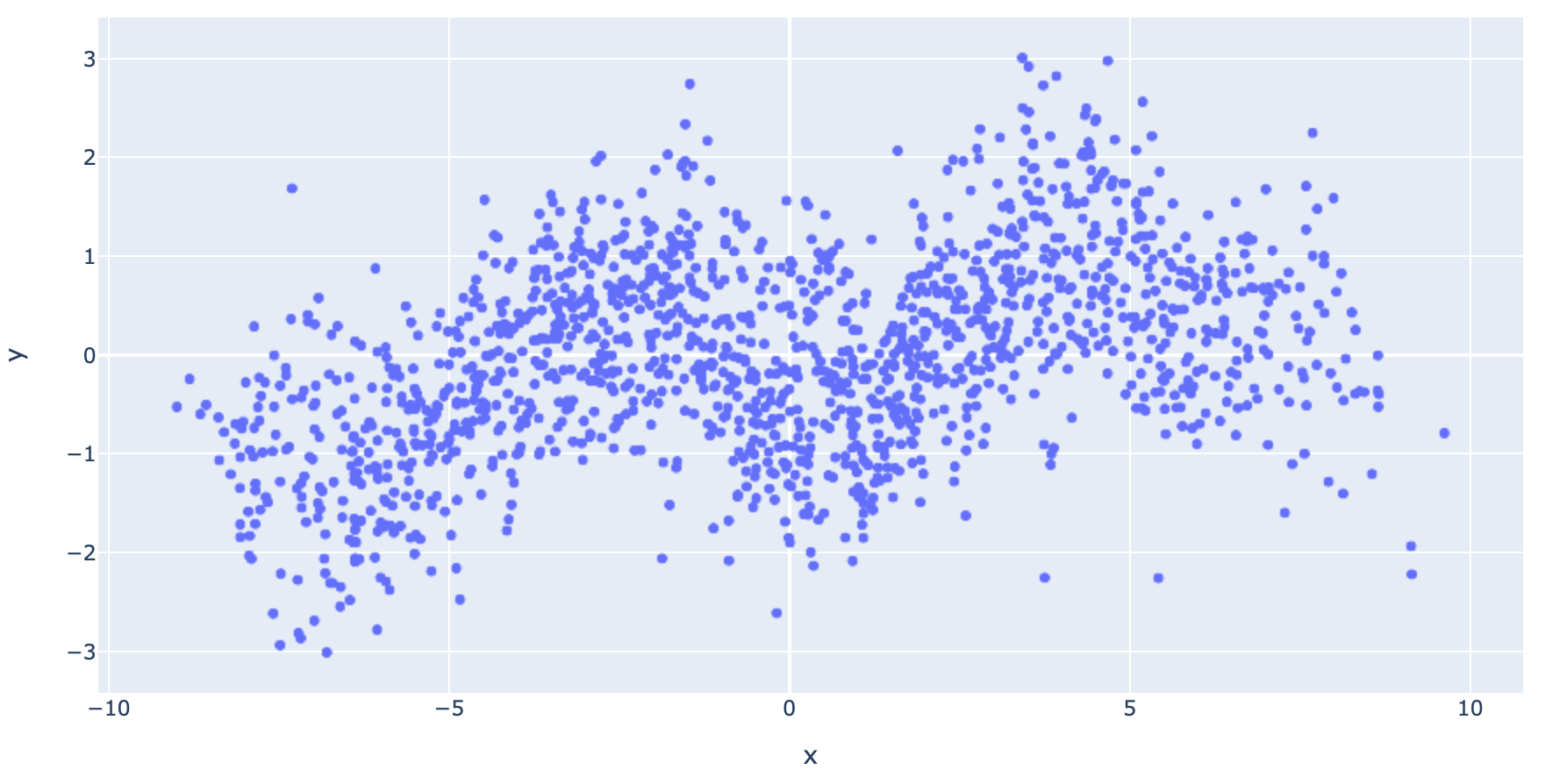

• นิยาม Model โดยกำหนด Activate Function ที่ Output Layer เป็นแบบ Linear ซึ่งจะทำให้ไม่มีการเปลี่ยนแปลงค่าใดๆ ก่อนจะนำออกจาก Output Layer ของ Model

model = tf.keras.Sequential()
model.add(tf.keras.Input(shape=(10,)))

model.add(tf.keras.layers.Dense(20, activation='relu', kernel_initializer='he_uniform'))
model.add(tf.keras.layers.Dense(1, activation='linear'))

• Compile Model โดยกำหนด Loss Function เป็น Mean Squared Error

opt = tf.keras.optimizers.SGD(learning_rate=0.01, momentum=0.9)
model.compile(loss='mean_squared_error', optimizer=opt)

• Train Model

history = model.fit(x_train, y_train, validation_data=(x_val, y_val), epochs=100, verbose=1)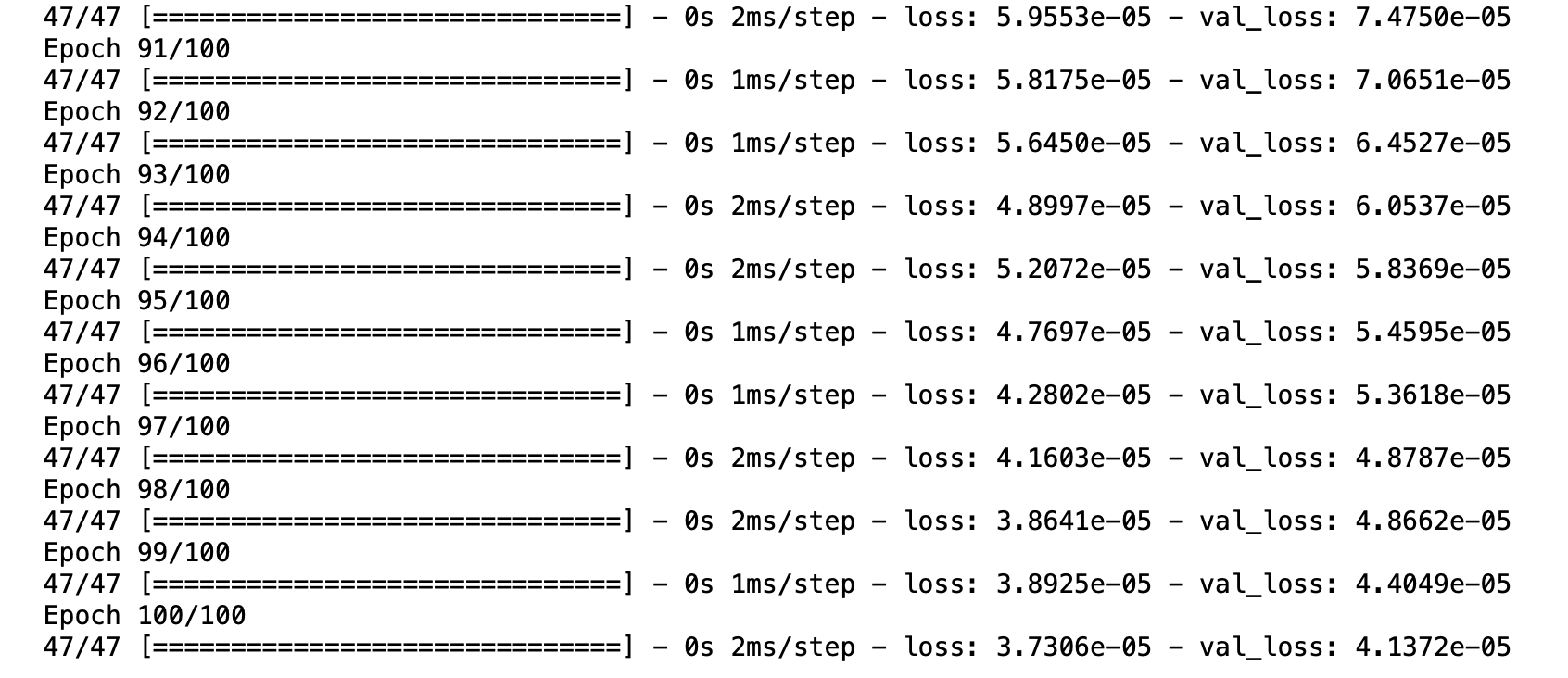

• Plot Loss

h1 = go.Scatter(y=history.history['loss'], 
                    mode="lines",
                    line=dict(
                        width=2,
                        color='blue'),
                        name="loss"
                   )
h2 = go.Scatter(y=history.history['val_loss'], 
                    mode="lines",
                    line=dict(
                        width=2,
                        color='red'),
                        name="val_loss"
                   )

data = [h1,h2]
layout1 = go.Layout(title='Loss',
                   xaxis=dict(title='epochs'),
                   yaxis=dict(title=''))
fig1 = go.Figure(data = data, layout=layout1)
plotly.offline.iplot(fig1)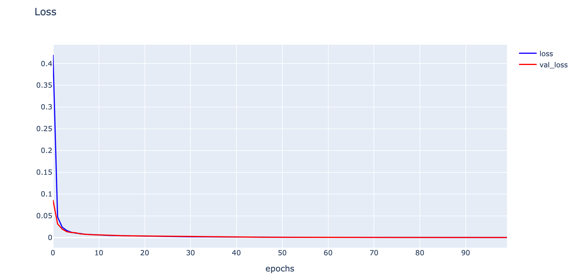

• Evaluate Model

train_mse = model.evaluate(x_train, y_train, verbose=0)
val_mse = model.evaluate(x_val, y_val, verbose=0)
print('Train: %.5f, Validation: %.5f' % (train_mse, val_mse))

Train: 0.00003, Validation: 0.00004

Mean Squared Logarithmic Error Loss

Mean Squared Logarithmic Error (MSLE) เป็นค่าที่แสดงถึงความแตกต่างสัมพัทธ์ (Relative Difference) ระหว่างผลเฉลยกับค่าที่เกิดจากการทำนายของ Model เช่น ถ้าเรามีค่าที่ต่างกัน 2 คู่ ได้แก่ 10 กับ 20 และ 1,000 กับ 2,000 ทั้ง 2 คู่จะมีความต่างกัน 2 เท่า Error แบบ MSLE จะให้ค่าที่ไม่แตกต่างกันมาก

ซึ่งหมายความว่า MSLE จะให้ความสำคัญกับความผิดพลาดทั้ง 2 แบบนี้ใกล้เคียงกัน เพราะมันมีสัดส่วนหรือเปอร์เซ็นต์ความต่างเท่ากัน ดังนั้น Model ที่ใช้ Mean Squared Logarithmic Error Loss จะไม่ถูกลงโทษอย่างหนักเมื่อมันทำความผิดร้ายแรงเหมือนกับ Model ที่ใช้ Mean Squared Error Loss

True value	Predicted value		MSE loss	MSLE loss
10		20			100		0.41813
1,000		2,000			1,000,000	0.48038

นอกจากนี้ Mean Squared Logarithmic Error Loss ยังลงโทษ Model ที่ให้ค่าในการทำนายน้อยกว่าค่าจริง (Underestimate) มากกว่าเมื่อ Model ให้ค่าในการทำนายมากกว่าค่าจริง (Overestimate) ดังตัวอย่างด้านล่าง

True value	Predicted value		MSE loss	MSLE loss
20		10			100		0.41813
20		30			100		0.15168

Example

Mean Squared Logarithmic Error Loss สามารถทำงานได้ดีกว่า Mean Squared Error Loss กับ Dataset อย่างเช่น Boston Housing ที่มีผลเฉลย หรือ Target เป็นมูลค่าราคากลางของบ้าน (MEDV: Median value of owner-occupied homes in $1000s) ซึ่งราคาจะขึ้นอยู่กับจำนวนห้องเฉลี่ยต่อหลังคาเรือน (RM: Average number of rooms per dwelling) และสัดส่วนของประชากรที่มีสถานะทางการศึกษาและเศรษฐกิจที่ต่ำกว่าค่าเฉลี่ย (LSTAT: Percentage of lower status of the population) นอกจากนี้ Mean Squared Logarithmic Error Loss ยังจะทำงานได้ดีกว่า Mean Squared Error Loss เมื่อเรานำมันมาใช้กับ Dataset ที่ไม่มีการทำ Scaling โดยผมจะขอยกตัวอย่างการ Train Model ด้วย Mean Squared Logarithmic Error Loss ดังต่อไปนี้

• Download Boston Housing Dataset
• Upload ขึ้น Google Colab
• อ่านไฟล์ BostonHousing.csv ที่ Download เข้า Dataframe

boston = pd.read_csv('BostonHousing.csv')
boston.head()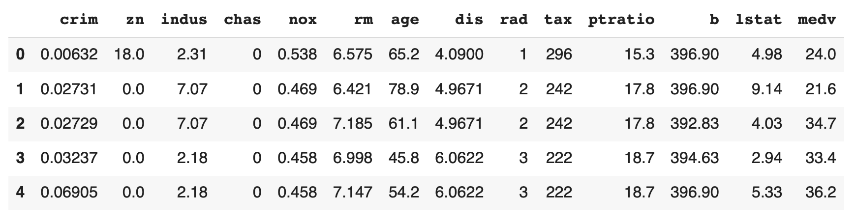

• เปลี่ยนชื่อ Column medev เป็น price (คูณ 1000 ดอลลาร์)

boston = boston_dataset.rename(columns={"medv": "price"})

• Plot Histogram ของ PRICE

sns.set(rc={'figure.figsize':(11,8)})
sns.histplot(boston['price'], bins=30, kde=True)
plt.show()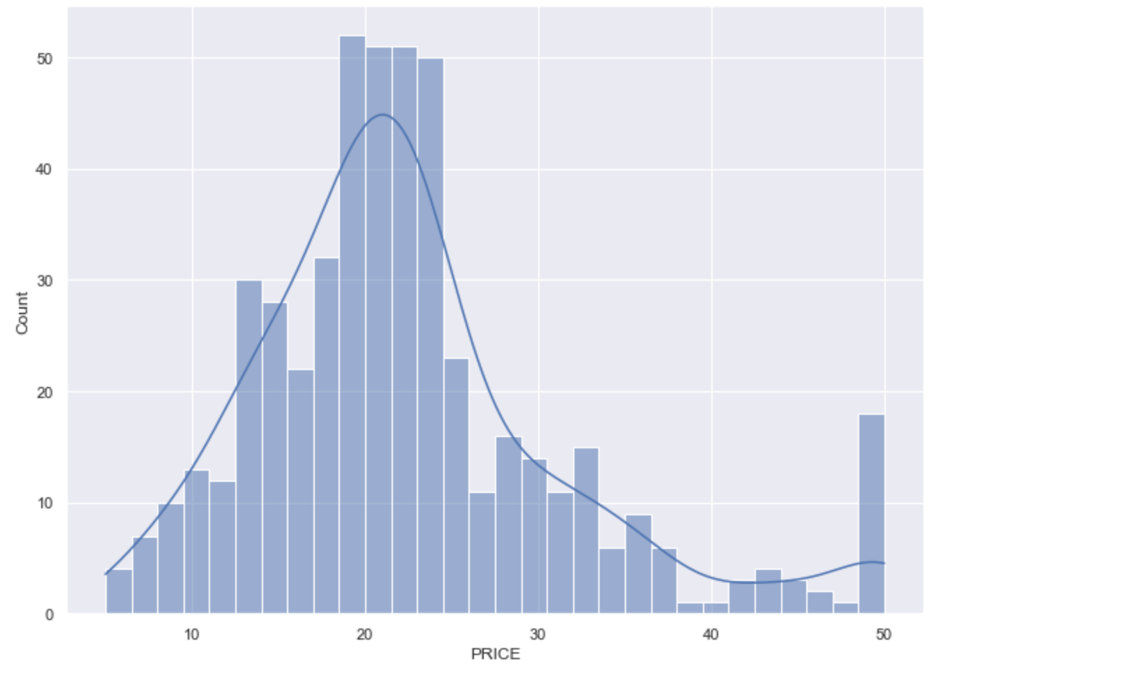

• Plot Correlation Matrix

correlation_matrix = boston.corr().round(3)

sns.heatmap(data=correlation_matrix, annot=True)
plt.savefig('correlation_matrix.jpeg', dpi=300)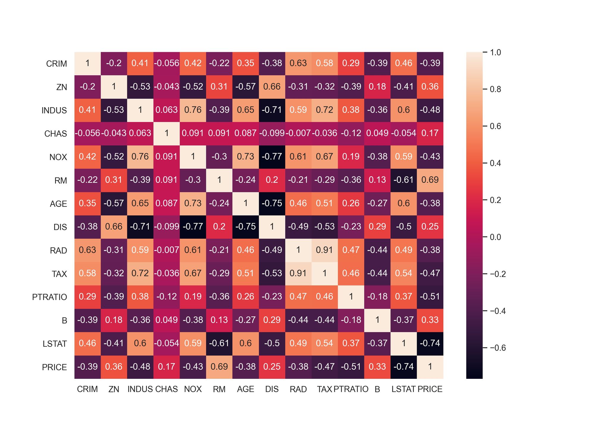

Correlation Matrix แสดงค่า Correlation Coefficient ซึ่งมีช่วงข้อมูลตั้งแต่ -1 ถึง 1 ที่แสดงความสัมพันธ์ของ Feature แบบ Linear Relationship โดยค่าเข้าใกล้ 1 หรือ -1 แสดงว่า Feature 2 ตัวมีความสัมพันธ์ที่เข้มแข็งในแบบ Positive Correlation หรือแบบ Negative Correlation ตามลำดับ

จาก Correlation Matrix เราจะเลือก RM และ LSTAT ซึ่งเป็น 2 Feature ที่มีความสัมพันธ์กับ PRICE มากที่สุด คือ มี Correlation Coefficient เท่ากับ 0.69 และ -0.74 เพื่อจะนำมาเป็น Input Data สำหรับการ Train Model

• ใช้ Scatter Plot แสดงความสัมพันธ์ระหว่าง RM กับ PRICE และระหว่าง LSTAT กับ PRICE

plt.figure(figsize=(25, 10))

features = ['rm', 'lstat']
target = boston['price']

for i, col in enumerate(features):
    plt.subplot(1, len(features) , i+1)
    x = boston[col]
    y = target
    plt.scatter(x, y, marker='o')
    plt.title(col)
    plt.xlabel(col)
    plt.ylabel('price')

plt.savefig('scatter.jpeg', dpi=300)

• สร้าง Input Data จาก Column LSTAT และ RM และผลเฉลยจาก Column PRICE

x = pd.DataFrame(np.c_[boston['lstat'], boston['rm']], columns = ['lstat','rm'])
y = boston['price']

x.shape, y.shape

((506, 2), (506,))

• แบ่งข้อมูลสำหรับ Train และ Test โดยการสุ่มในสัดส่วน 80:20

x_train, x_val, y_train, y_val = train_test_split(x, y, test_size = 0.2, random_state=5)

x_train.shape, x_val.shape, y_train.shape, y_val.shape

((404, 2), (102, 2), (404,), (102,))

• นิยาม Model โดยกำหนด Activate Function ที่ Output Layer เป็นแบบ Linear ซึ่งจะทำให้ไม่มีการเปลี่ยนแปลงค่าใดๆ ก่อนจะนำออกจาก Output Layer ของ Model

model = tf.keras.Sequential()
model.add(tf.keras.Input(shape=(2,)))
model.add(tf.keras.layers.Dense(20, activation='relu', kernel_initializer='he_uniform'))
model.add(tf.keras.layers.Dense(1, activation='linear'))

• Compile Model โดยกำหนด Loss Function เป็น Mean Squared Error เพื่อใช้ในการเปรียบเทียบกับ Mean Squared Logarithmic Error ในการ Train ครั้งต่อไป

opt = tf.keras.optimizers.SGD(learning_rate=0.01, momentum=0.9)
model.compile(loss='mean_squared_error', optimizer=opt)

• Train Model

history = model.fit(x_train, y_train, validation_data=(x_val, y_val), epochs=200, verbose=1)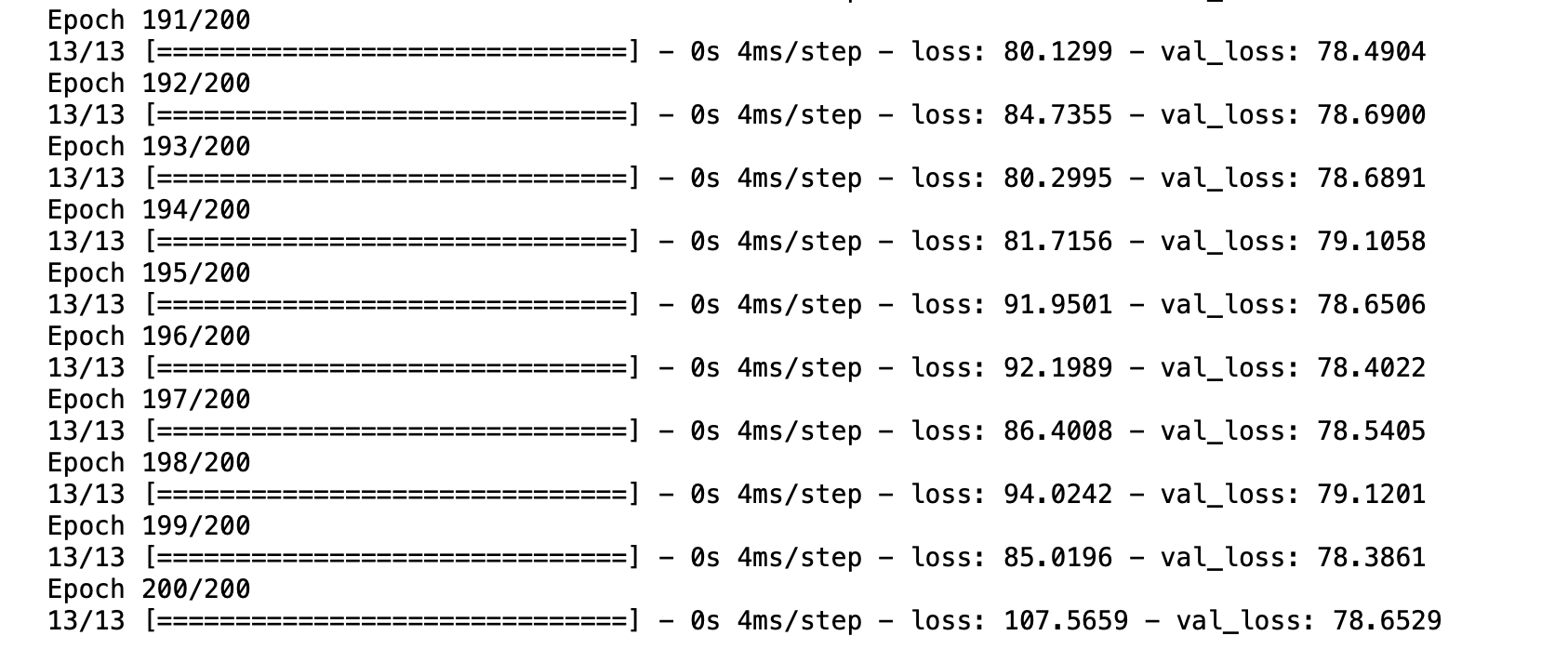

• Plot Loss

h1 = go.Scatter(y=history.history['loss'], 
                    mode="lines",
                    line=dict(
                        width=2,
                        color='blue'),
                        name="loss"
                   )
h2 = go.Scatter(y=history.history['val_loss'], 
                    mode="lines",
                    line=dict(
                        width=2,
                        color='red'),
                        name="val_loss"
                   )

data = [h1,h2]
layout1 = go.Layout(title='Loss',
                   xaxis=dict(title='epochs'),
                   yaxis=dict(title=''))
fig1 = go.Figure(data = data, layout=layout1)
plotly.offline.iplot(fig1)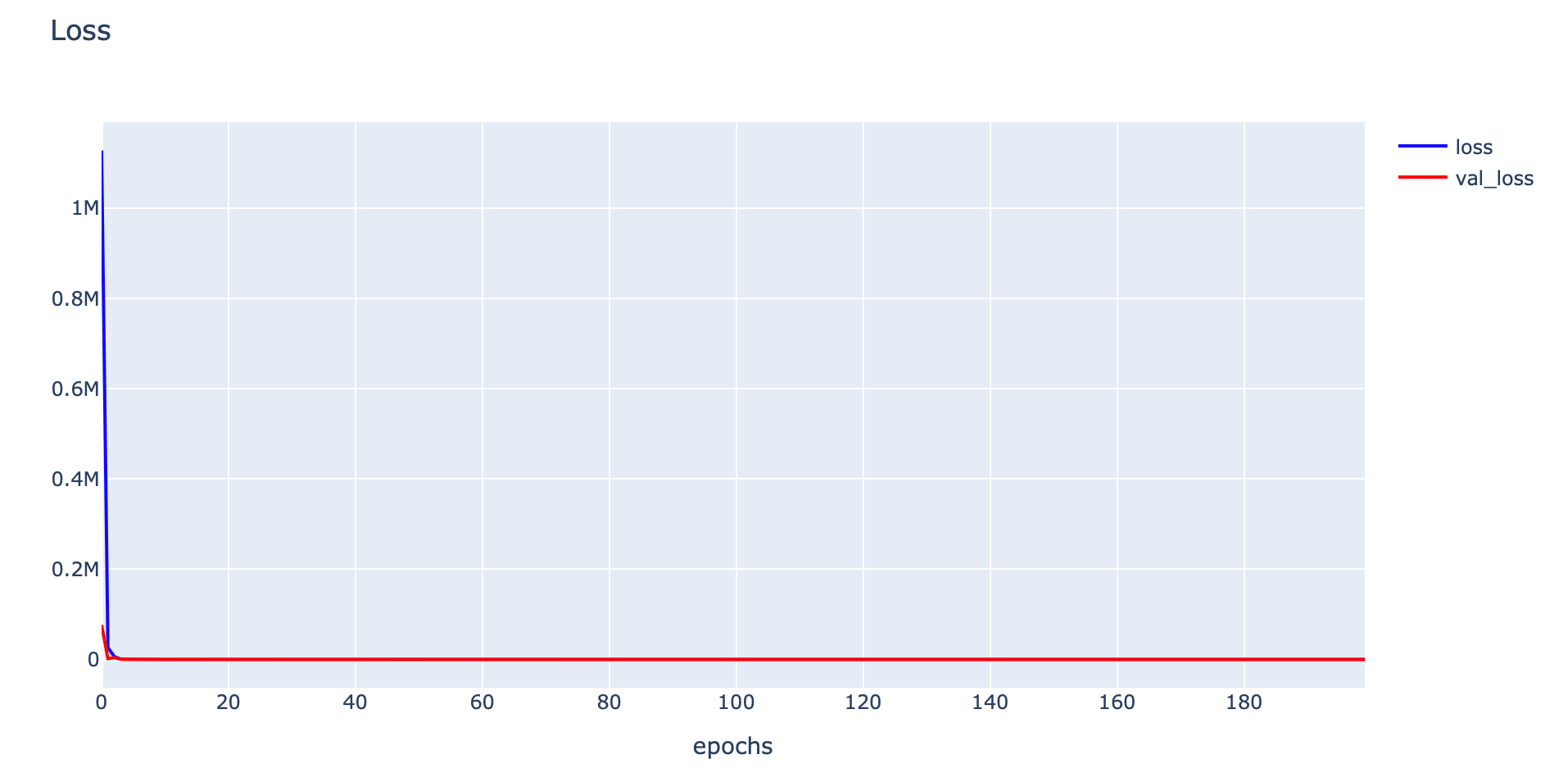

• Evaluate Model

train_mse = model.evaluate(x_train, y_train, verbose=0)
val_mse = model.evaluate(x_val, y_val, verbose=0)
print('Train: %.5f, Validation: %.5f' % (train_mse, val_mse))

Train: 85.90284, Validation: 78.65289

• นิยาม Model โดยกำหนด Activate Function ที่ Output Layer เป็นแบบ Linear ซึ่งจะทำให้ไม่มีการเปลี่ยนแปลงค่าใดๆ ก่อนจะนำออกจาก Output Layer ของ Model

model = tf.keras.Sequential()
model.add(tf.keras.Input(shape=(2,)))
model.add(tf.keras.layers.Dense(20, activation='relu', kernel_initializer='he_uniform'))
model.add(tf.keras.layers.Dense(1, activation='linear'))

• Compile Model โดยกำหนด Loss Function เป็น Mean Squared Logarithmic Error

opt = tf.keras.optimizers.SGD(learning_rate=0.01, momentum=0.9)

model.compile(loss='mean_squared_logarithmic_error', optimizer=opt, metrics=['mse'])

• Train Model

history = model.fit(x_train, y_train, validation_data=(x_val, y_val), epochs=200, verbose=1)

• Plot Loss

h1 = go.Scatter(y=history.history['loss'], 
                    mode="lines",
                    line=dict(
                        width=2,
                        color='blue'),
                        name="loss"
                   )
h2 = go.Scatter(y=history.history['val_loss'], 
                    mode="lines",
                    line=dict(
                        width=2,
                        color='red'),
                        name="val_loss"
                   )

data = [h1,h2]
layout1 = go.Layout(title='Loss',
                   xaxis=dict(title='epochs'),
                   yaxis=dict(title=''))
fig1 = go.Figure(data = data, layout=layout1)
plotly.offline.iplot(fig1)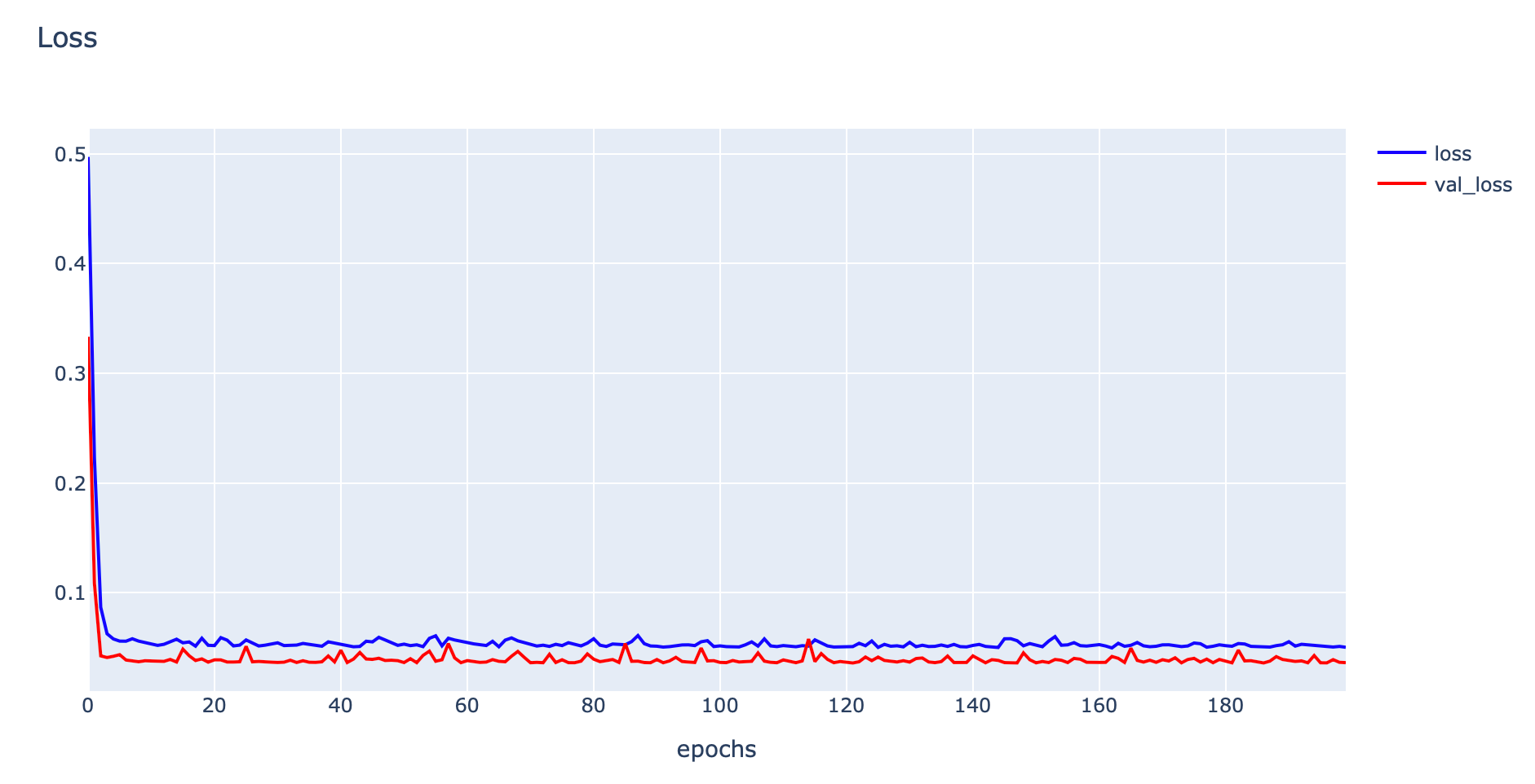

• Evaluate Model

train_msle = model.evaluate(x_train, y_train, verbose=0)
val_msle = model.evaluate(x_val, y_val, verbose=0)
print('MSLE Train: %.5f, Validation: %.5f' % (train_msle[0], val_msle[0]))
print('MSE Train: %.5f, Validation: %.5f' % (train_msle[1], val_msle[1]))

MSLE Train: 0.04960, Validation: 0.03616
MSE Train: 24.23595, Validation: 15.43487

จากการทดลอง พบว่า Model ที่ใช้ Mean Squared Logarithmic Error Loss จะมีประสิทธิภาพดีกว่า Model ที่ใช้ Mean Squared Error Loss เมื่อ Train ด้วย Boston Housing Dataset โดยไม่มีการทำ Scaling ดังข้อมูลสรุปด้านล่าง

Loss Function				val_mse		
mean_squared_error			78.65
mean_squared_logarithmic_error		15.43

สำหรับการทดลองที่ผ่านมา เราได้เห็นตัวอย่างการใช้งาน Mean Squared Error Loss และ Mean Squared Logarithmic Error Loss กับ Regression Model ที่มีการรับค่าและทำนายค่าเป็นเลขทศนิยมกันแล้ว ในลำดับต่อไป เราจะได้ทดลองใช้งาน Loss Function ตัวใหม่ที่ชื่อ Mean Absolute Error Loss กับ Autoencoder Model ซึ่งมีการรับค่าและทำนายค่าเป็น Pixel ของรูปภาพกันบ้าง

Autoencoder Loss Function

Autoencoder เป็น Neural Network ที่มีโครงสร้างคล้ายรูปนาฬิกาทราย ซึ่งส่วนปลายทั้งสองข้างกว้าง แต่ตรงกลางของ Model แคบ ดังภาพด้านล่าง

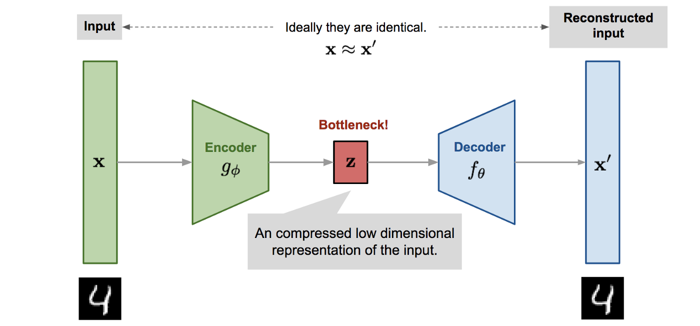
จากภาพ ส่วนปลายด้านที่ติดกับ Input Layer คือ Encoder Function มีหน้าที่แปลง Input Data X เป็น Latent Vector Z ขณะที่ส่วนปลายอีกด้าน คือ Decoder Function ทำหน้าที่แปลง Latent Vector Z กลับเป็น Output Data X'

ซึ่งในระหว่างการ Train Autoencoder กับ Image Dataset, Encoder จะเรียนรู้ที่จะสรุปย่อ Information (Latent Vector Z) จาก Input Image และ Decoder จะเรียนรู้ที่จะแปลง Latent Vector Z กลับเป็น Output Image ที่ปลายอีกด้านของ Model

เราจะทดลองใช้ Autoencoder เพื่อลดสัญญาณรบกวนของภาพที่นำมาจาก Mnist Dataset โดยใช้ Loss Function 2 แบบ ได้แก่ 1) Mean Squared Error Loss และ 2) Mean Absolute Error Loss ซึ่ง Loss Function ทั้ง 2 ตัว จะให้ประสิทธิภาพในการลดสัญญาณรบกวนที่แตกต่างกัน

Mean Absolute Error Loss

Mean Absolute Error (MAE) คือ ค่าเฉลี่ยของผลต่างสัมบูรณ์ ระหว่างผลเฉลยกับค่าที่เกิดจากการทำนายของ Model โดย Model ที่ใช้ MAE เป็น Loss Function จะทนต่อ Data ที่มี Outlier ได้มากกว่า Model ที่ใช้ MSE เป็น Loss Function

เช่นถ้า 90% ของ Dataset มีผลเฉลย หรือ Target เท่ากับ 130 ส่วนที่เหลืออีก 10% มีผลเฉลยในช่วง 0 - 30 แล้ว Model ที่ใช้ MAE จะทำนายค่าเป็น 130 ได้อย่างถูกต้อง แต่มันจะให้น้ำหนักน้อยกับส่วนที่เหลืออีก 10% ที่เป็น Outlier เมื่อเทียบกับ MSE

ดังนั้นถ้า Data ของเรามี Outlier ที่แสดงถึงความผิดปกติ (Anomaly) ซึ่งเป็นสิ่งสำคัญที่ Model ควรจะ Detect เราควรเลือกใช้ MSE เป็น Loss Function แต่ถ้า Data ของเรามี Outlier ที่เป็นเพียงความเสียหายของข้อมูล เราควรเลือกใช้ MAE แทน MSE ครับ

Example

Mean Absolute Error Loss สามารถทำงานได้ดีกว่า Mean Squared Error Loss กับ Mnist Dataset ในการลดสัญญาณรบกวนของภาพ ด้วย Autoencoder Model โดย Output Image ที่ได้จาก Mean Absolute Error Loss จะมีความคมชัดกว่า Output Image ที่ได้จาก Mean Squared Error Loss ตามตัวอย่างดังต่อไปนี้

• Load Mnist Dataset และทำ Scaling Data

(train_images, train_labels), (test_images, test_labels) = mnist.load_data()
train_images = train_images.reshape((60000, 28, 28, 1))
test_images = test_images.reshape((10000, 28, 28, 1))

train_images, test_images = train_images / 255.0, test_images / 255.0

• Plot รูปตัวอย่าง

for i in range(9):
    plt.subplot(330 + 1 + i)    
    img = train_images[i].reshape(train_images[0].shape[0], train_images[0].shape[1])
    plt.axis('off')
    plt.imshow(img, cmap=plt.get_cmap('gray'))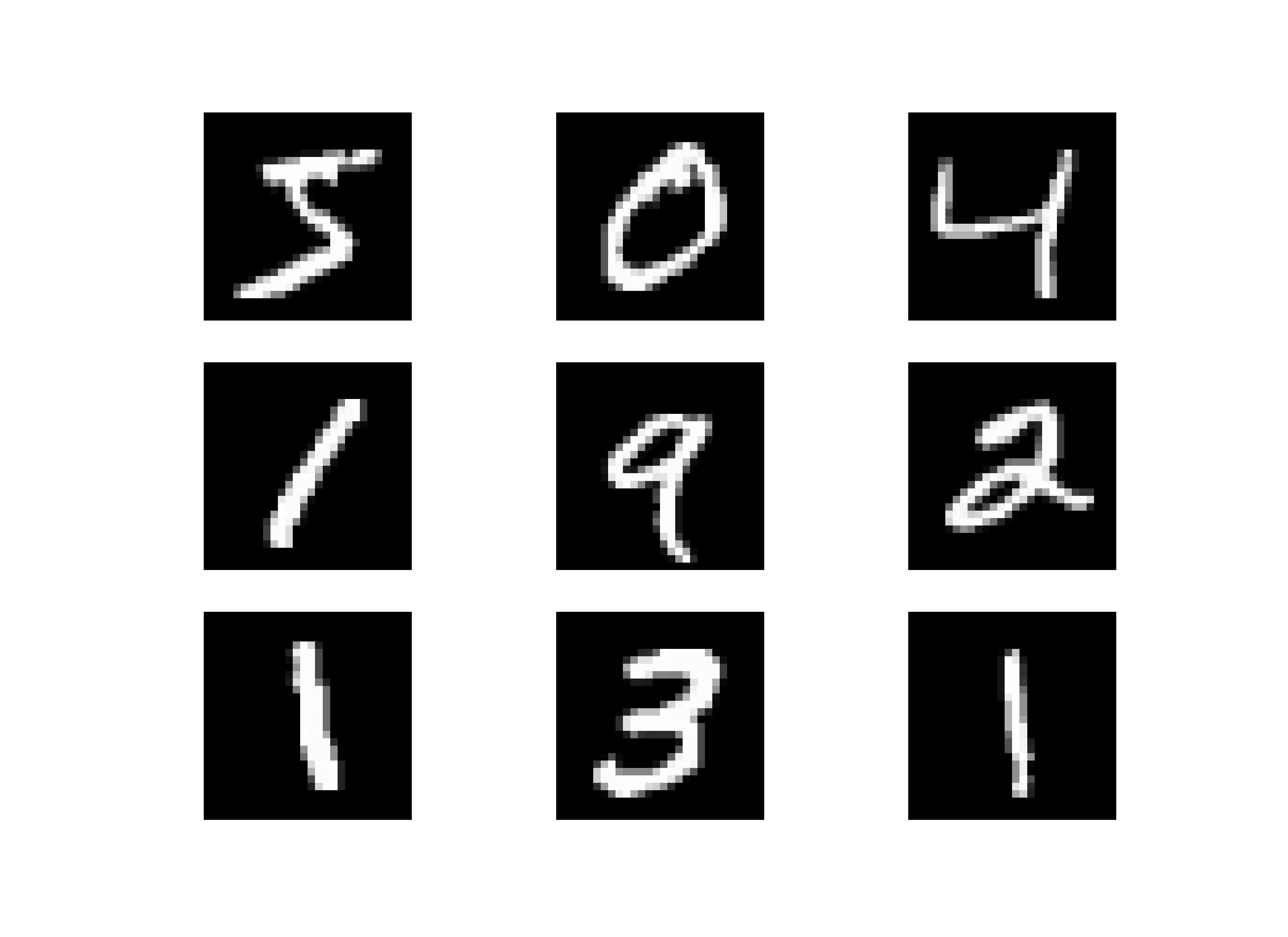

• สร้างสัญญาณรบกวนในภาพสำหรับการ Train และ Test

noise_factor = 0.5
x_train_noisy = train_images + noise_factor * np.random.normal(loc=0.0, scale=1.0, size=train_images.shape) 
x_test_noisy = test_images + noise_factor * np.random.normal(loc=0.0, scale=1.0, size=test_images.shape) 

x_train_noisy = np.clip(x_train_noisy, 0., 1.)
x_test_noisy = np.clip(x_test_noisy, 0., 1.)

• Plot ภาพที่มีสัญญาณรบกวน จาก Train Dataset

for i in range(9):
    plt.subplot(330 + 1 + i)    
    
    img = x_train_noisy[i].reshape(x_train_noisy[0].shape[0], x_train_noisy[0].shape[1])
    plt.axis('off')
    plt.imshow(img, cmap=plt.get_cmap('gray'))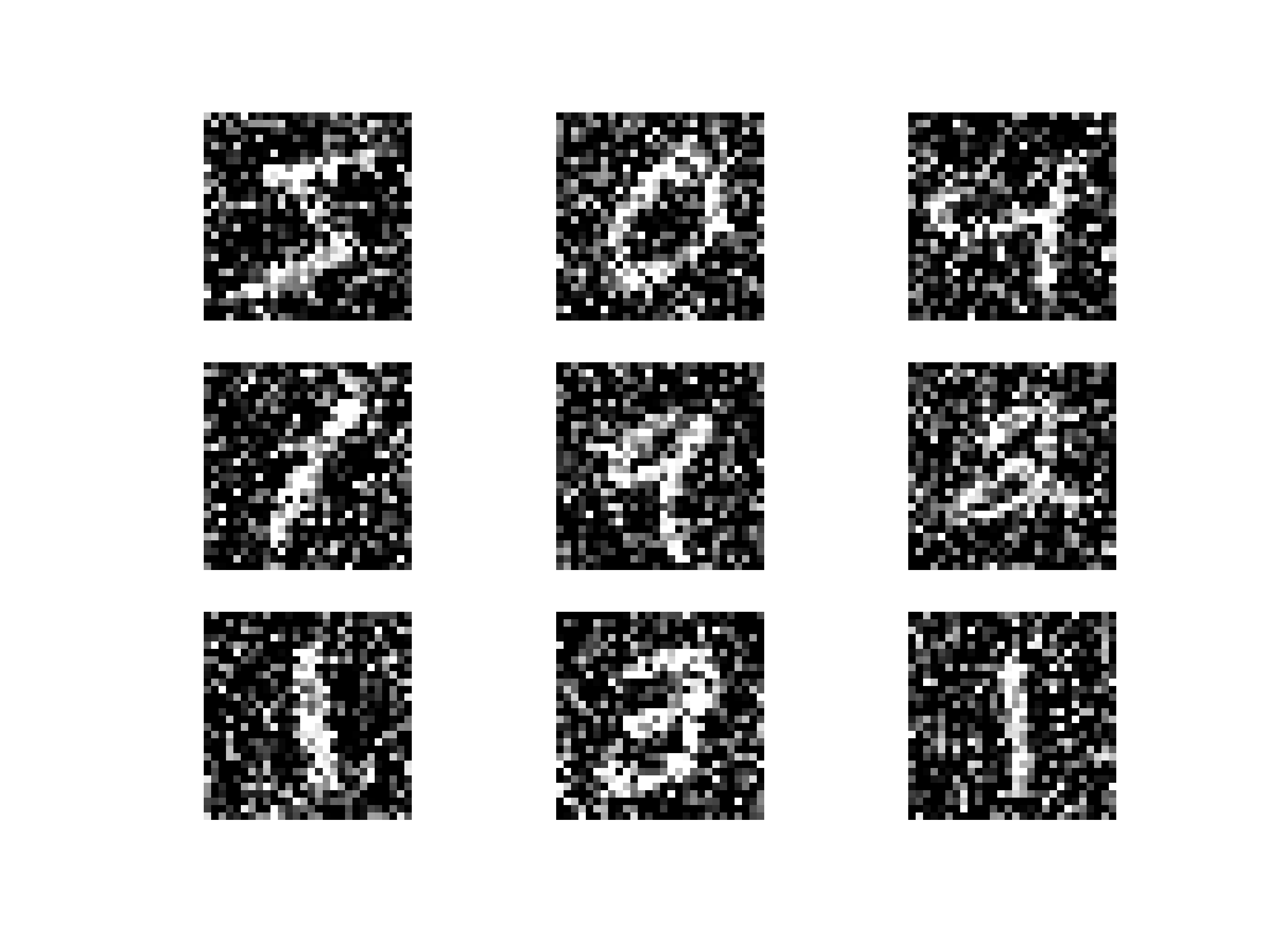

• นิยาม Model แบบ Autoencoder โดยกำหนด Activate Function เป็น ReLu และ Sigmoid

#Encoder
inp = tf.keras.layers.Input((28, 28,1))
e = tf.keras.layers.Conv2D(32, (3, 3), activation='relu')(inp)
e = tf.keras.layers.BatchNormalization()(e)

e = tf.keras.layers.MaxPooling2D((2, 2))(e)
e = tf.keras.layers.Conv2D(64, (3, 3), activation='relu')(e)
e = tf.keras.layers.BatchNormalization()(e)

e = tf.keras.layers.MaxPooling2D((2, 2))(e)
e = tf.keras.layers.Conv2D(64, (3, 3), activation='relu')(e)
e = tf.keras.layers.BatchNormalization()(e)

l = tf.keras.layers.Flatten()(e)
l = tf.keras.layers.Dense(49, activation='relu')(l)

#DECODER
d = tf.keras.layers.Reshape((7,7,1))(l)
d = tf.keras.layers.Conv2DTranspose(64,(3, 3), strides=2, activation='relu', padding='same')(d)
d = tf.keras.layers.BatchNormalization()(d)
d = tf.keras.layers.Conv2DTranspose(64,(3, 3), strides=2, activation='relu', padding='same')(d)
d = tf.keras.layers.BatchNormalization()(d)
d = tf.keras.layers.Conv2DTranspose(32,(3, 3), activation='relu', padding='same')(d)
decoded = tf.keras.layers.Conv2D(1, (3, 3), activation='sigmoid', padding='same')(d)
ae = tf.keras.Model(inp, decoded)

ae.summary()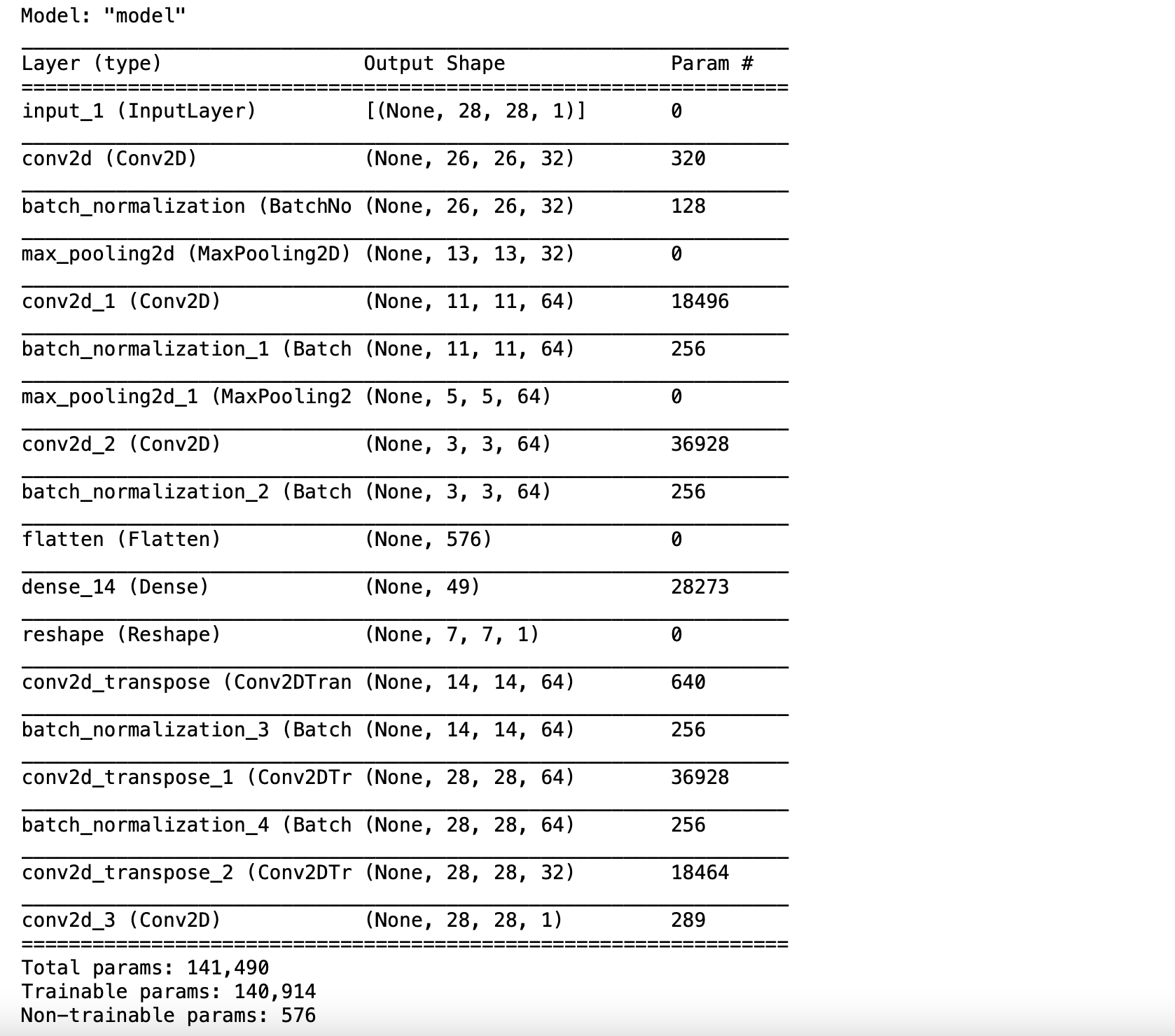

• Compile Model โดยใช้ Mean Squared Error Loss

ae.compile(optimizer='adam', loss='mse')

• Train Model

ae.fit(x_train_noisy, train_images, epochs=2, verbose=1)

• เรียกใช้ฟังก์ชัน Predict โดยรับ Input Image ที่มีสัญญาณรบกวน

test_prediction = ae.predict(x_test_noisy, verbose=1, batch_size=100)

100/100 [==============================] - 9s 92ms/step

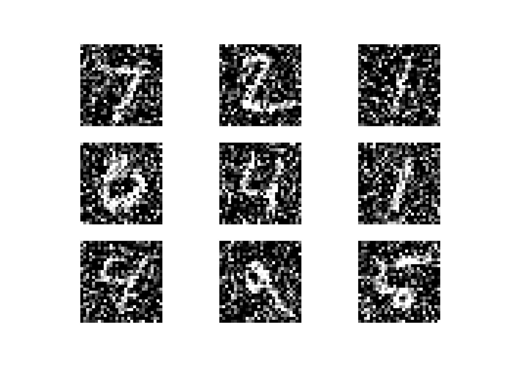
• Plot ภาพที่มีสัญญาณรบกวนจาก Test Dataset

for i in range(9):
    plt.subplot(330 + 1 + i)    
    
    img = x_test_noisy[i].reshape(x_test_noisy[0].shape[0], x_test_noisy[0].shape[1])
    plt.axis('off')
    plt.imshow(img, cmap=plt.get_cmap('gray'))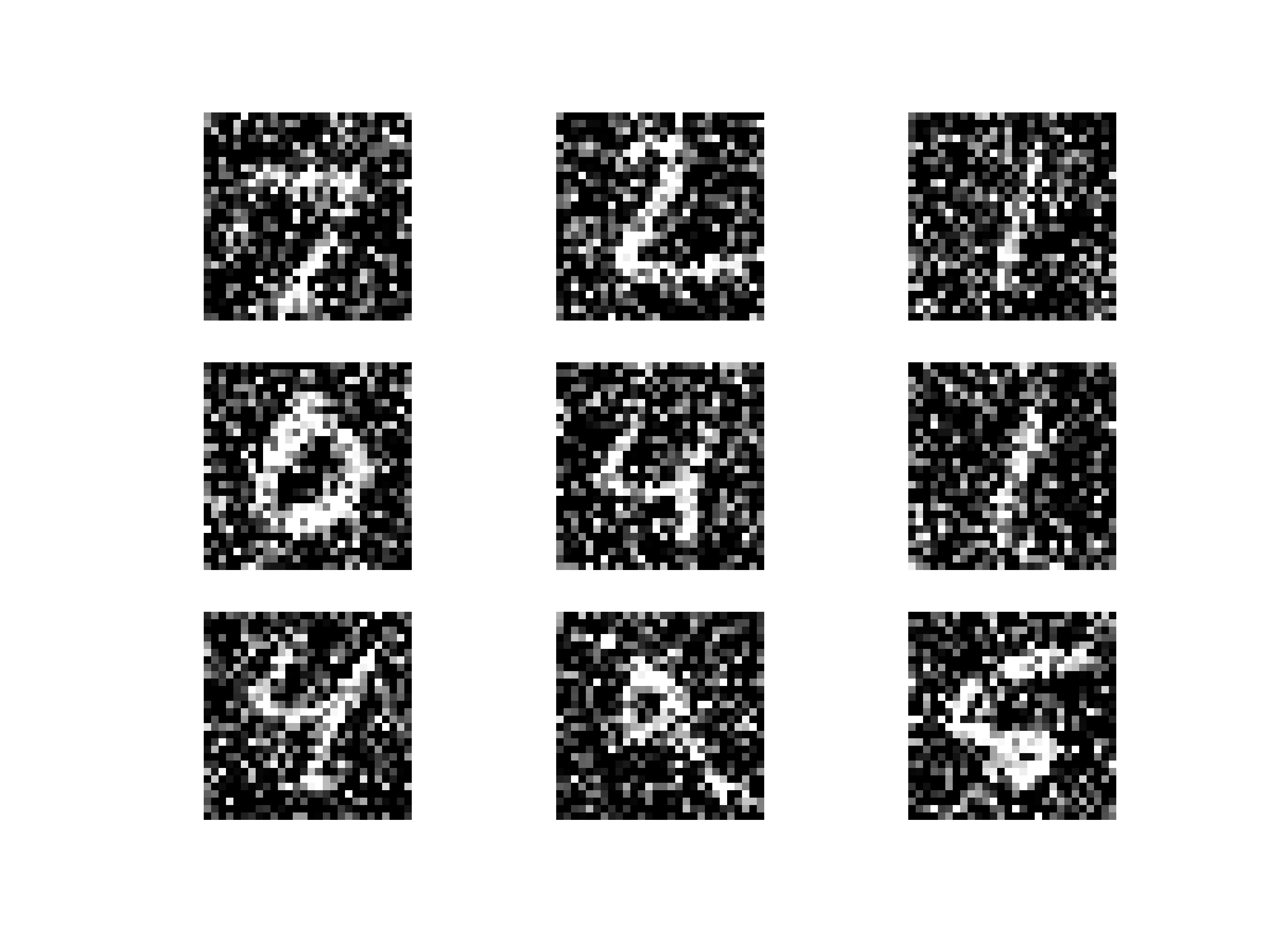

• Plot ภาพที่ลดสัญญาณรบกวนแล้ว

for i in range(9):
    plt.subplot(330 + 1 + i)    
    
    x = test_prediction[i].reshape(28,28)
    plt.axis('off')
    plt.grid(False)
    plt.imshow(x, cmap=plt.get_cmap('gray'))

• นิยาม Model แบบ Autoencoder โดยกำหนด Activate Function เป็น ReLu และ Sigmoid

#Encoder
inp = tf.keras.layers.Input((28, 28,1))
e = tf.keras.layers.Conv2D(32, (3, 3), activation='relu')(inp)
e = tf.keras.layers.BatchNormalization()(e)

e = tf.keras.layers.MaxPooling2D((2, 2))(e)
e = tf.keras.layers.Conv2D(64, (3, 3), activation='relu')(e)
e = tf.keras.layers.BatchNormalization()(e)

e = tf.keras.layers.MaxPooling2D((2, 2))(e)
e = tf.keras.layers.Conv2D(64, (3, 3), activation='relu')(e)
e = tf.keras.layers.BatchNormalization()(e)

l = tf.keras.layers.Flatten()(e)
l = tf.keras.layers.Dense(49, activation='relu')(l)

#Decoder
d = tf.keras.layers.Reshape((7,7,1))(l)
d = tf.keras.layers.Conv2DTranspose(64,(3, 3), strides=2, activation='relu', padding='same')(d)
d = tf.keras.layers.BatchNormalization()(d)
d = tf.keras.layers.Conv2DTranspose(64,(3, 3), strides=2, activation='relu', padding='same')(d)
d = tf.keras.layers.BatchNormalization()(d)
d = tf.keras.layers.Conv2DTranspose(32,(3, 3), activation='relu', padding='same')(d)
decoded = tf.keras.layers.Conv2D(1, (3, 3), activation='sigmoid', padding='same')(d)
ae = tf.keras.Model(inp, decoded)

• Compile Model โดยใช้ Mean Absolute Error Loss

ae.compile(optimizer="adam", loss="mae")

• Train Model

ae.fit(x_train_noisy, train_images, epochs=2, verbose=1)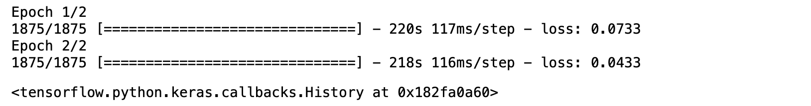

• เรียกใช้ฟังก์ชัน Predict โดยรับ Input Image ที่มีสัญญาณรบกวน

test_prediction = ae.predict(x_test_noisy, verbose=1, batch_size=100)

100/100 [==============================] - 10s 94ms/step

• Plot ภาพที่ลดสัญญาณรบกวนแล้ว

for i in range(9):
    plt.subplot(330 + 1 + i)    
    
    x = test_prediction[i].reshape(28,28)
    plt.axis('off')
    plt.imshow(x, cmap=plt.get_cmap('gray'))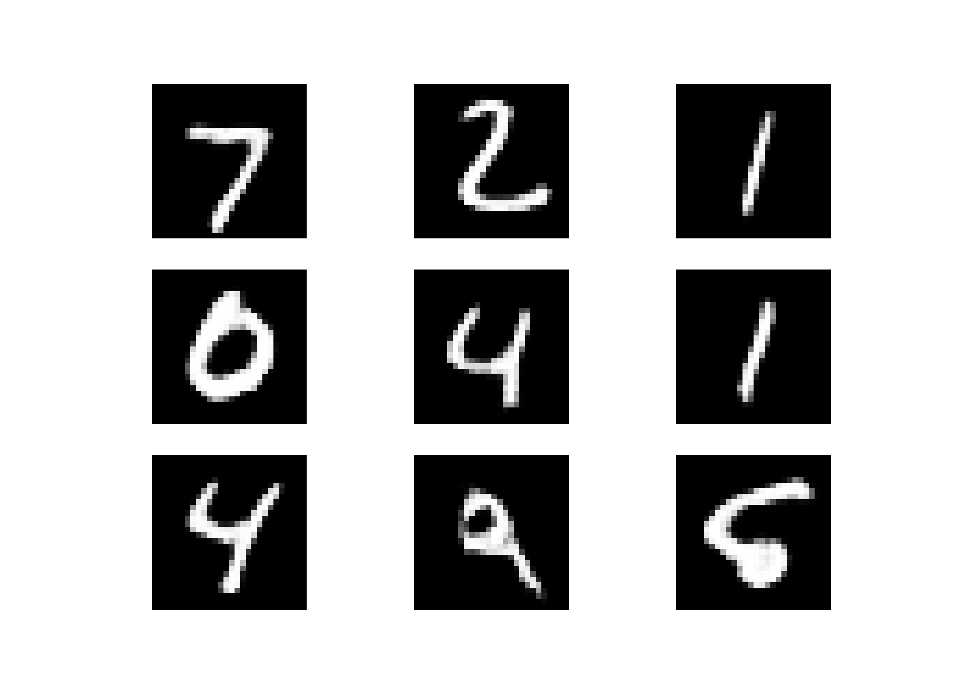

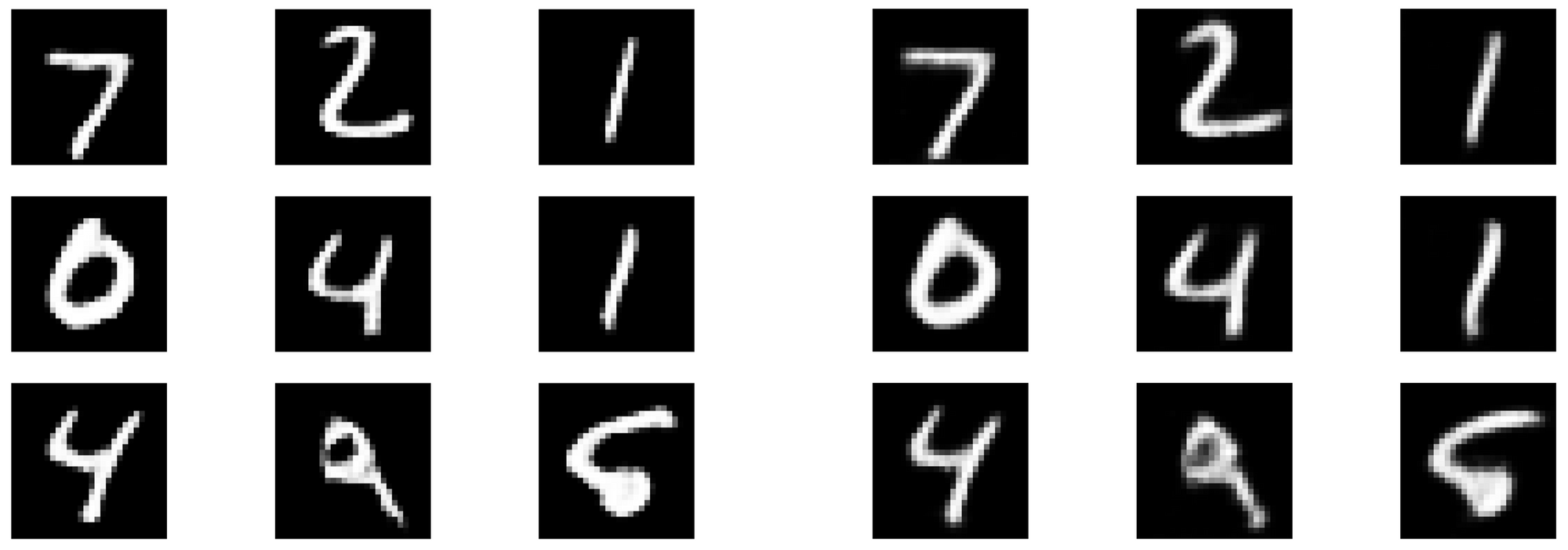
จากภาพที่ลดสัญญาณรบกวนด้านบนด้วย Autoencoder พบว่า Model ที่ใช้ Mean Absolute Error Loss จะให้ภาพที่มีความคมชัดกว่า Model ที่ใช้ Mean Squared Error Loss ครับ

• การเลือกใช้ Loss Function ในการพัฒนา Deep Learning Model (ตอนที่ 1)
• การเลือกใช้ Loss Function ในการพัฒนา Deep Learning Model (ตอนที่ 2)