Evaluation Metrics for Classification Model


บทความโดย ผศ.ดร.ณัฐโชติ พรหมฤทธิ์
ภาควิชาคอมพิวเตอร์
คณะวิทยาศาสตร์
มหาวิทยาลัยศิลปากร
Accuracy และ Loss เป็นเครื่องมือมาตรฐานที่ใช้ในการวัด (Metric) หรือประเมิน Classification Model แต่การจะประเมิน Model เพียงจาก Accuracy และ Loss อาจทำให้เกิดการเข้าใจผิดจนเกิดการเลือก Model ที่ไม่ดีมาแทน Model ที่ดี หรืออาจทำให้ไม่สามารถแก้ปัญหาในระหว่างการพัฒนา Model ได้อย่างตรงจุด
บทความนี้ ผู้อ่านจะได้เห็นการใช้งานเครื่องมือต่างๆ ได้แก่ Confusion Matrix, Precision, Recall, F1-score, ROC (Receiver Operating Characteristics) และ AUC (Area Under The Curve) ในการประเมิน Binary Classification Model ซึ่งเมื่อได้ทำความเข้าใจแนวคิดหลักๆ ของเครื่องมือเหล่านี้ดีแล้ว เราจะนำมันไปประยุกต์ใช้สำหรับการประเมิน Multi-Class Classification Model ในหัวข้อสุดท้ายของบทความ
Binary Classification Evaluation
สมมติว่ามีบุคคล 2 กลุ่ม กลุ่มหนึ่งติดเชื้อไวรัส โคโรนา อีกกลุ่มไม่ติดเชื้อ ซึ่งสามารถวินิจฉัยได้จากภาพ X-ray ปอดของพวกเขา ในการแยกประเภทบุคคลเป็น 2 กลุ่ม คือ ปอดติดเชื้อ และปอดไม่ติดเชื้อ เราจะพัฒนา Model แบบ Binary Classification ครับ
Binary Classification เป็น Model ที่มีการกำหนด Label หรือ Class เพียง 2 Class คือ เป็น Class 0 (ไม่ติดเชื้อ) กับเป็น Class 1 (ติดเชื้อ) ซึ่งผลลัพธ์จากการทำนายของ Model จะบอกว่ามีโอกาสที่จะเป็น Class 1 กี่เปอร์เซ็นต์
เพื่อจะทำให้ Neural Network Model ทำนายผลออกมาเป็นค่าความเชื่อมั่นซึ่งมีค่าตั้งแต่ 0-1 เราจะต้องคอนฟิก Activate Function ใน Output Layer แบบ Sigmoid
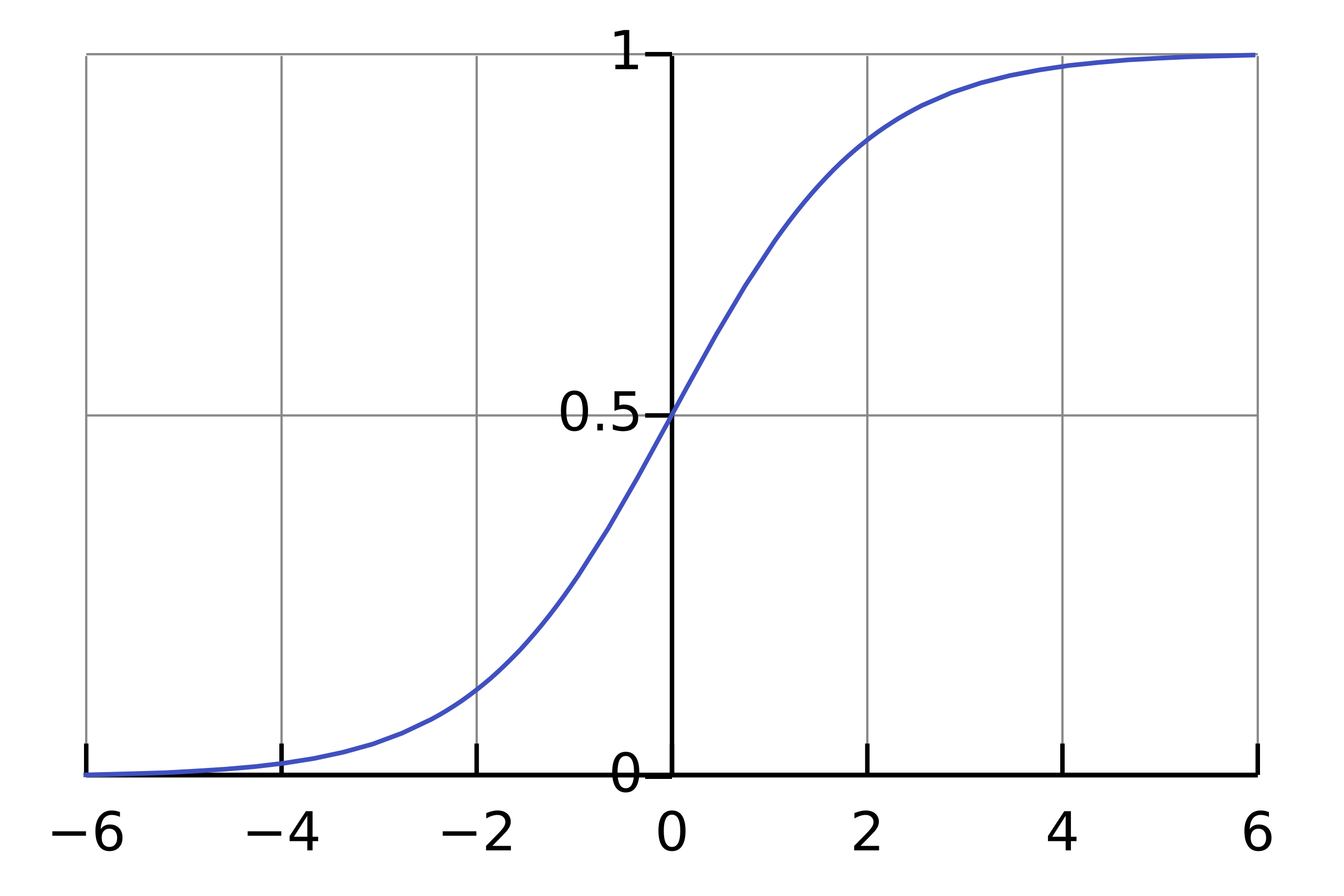
ซึ่งโดย Default แล้ว Binary Classification Model จะทำนายว่าเป็น Class 1 เมื่อมีค่าความเชื่อมั่นมากกว่า 0.5
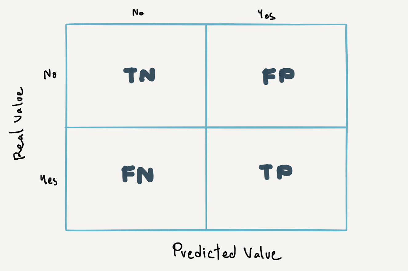
เราเรียกผลการทำนายกลุ่มคนที่ติดเชื้อ ที่ Model ทำนายถูกเป็นติดเชื้อว่า True Possitive (TP) และเรียกผลการทำนายกลุ่มคนที่ไม่ติดเชื้อ ที่ Model ทำนายถูกเป็นไม่ติดเชื้อว่า True Negative (TN)
อย่างไรก็ตาม อาจจะมีภาพ X-ray ปอดบางภาพที่ดูเหมือนไม่ติดเชื้อ แต่เกิดการติดเชื้อ (False Negative:FN) และภาพปอดที่ดูเหมือนติดเชื้อ แต่จริงๆ แล้วไม่ติด (False Positive:FP) ได้เช่นกัน ซึ่งในกรณีของการทำนายว่ามีการติดเชื้อไวรัสโคโรนาหรือไม่ เราจะซีเรียสกับผลของการทำนายว่าไม่ติดเชื้อแต่จริงๆ แล้วติดเชื้อ (FN) มากกว่าการทำนายว่าติดเชื้อ แต่จริงๆ แล้วไม่ติด (FP) เพราะถ้าไม่ได้รับการดูแลรักษาที่ถูกต้องรวดเร็ว จะส่งผลให้เชื้อไวรัสแพร่กระจายเป็นอันตรายถึงชีวิต รวมทั้งคนที่ติดเชื้อเหล่านั้นอาจไม่ระมัดระวังตัว จนไปแพร่เชื้อให้กับคนใกล้ชิดได้ครับ
Confusion Matrix, Recall และ Precision
เราจะวางผลการทำนายในแบบต่างๆ ลงในตาราง Confusion Matrix ดังต่อไปนี้
ซึ่งจาก Confusion Matrix จะสามารถคำนวนค่า Recall หรือ Sensitivity หรือ True Positive Rate ที่แสดงถึงประสิทธิภาพของ Model เมื่อเราซีเรียสผลการทำนายแบบ False Negative ดังสมการด้านล่าง
Recall หรือ Sensitivity หรือ True Positive Rate = TP/(TP+FN)และจะสามารถคำนวนณค่า Precision ที่แสดงถึงประสิทธิภาพของ Model เมื่อเราซีเรียสผลการทำนายแบบ False Positive เช่นในกรณีของการทำนายว่าเป็น Junk Mail หรือไม่เป็น Junk Mail ซึ่งเมื่อเกิดผลการทำนายแบบ False Positive หรือทำนาย Email ปกติเป็น Junk Mail จะทำให้ผู้รับพลาดการติดต่อเรื่องสำคัญได้ครับ
Precision = TP/(TP+FP)อย่างไรก็ตามถ้าเรามีการพัฒนา Model แบบที่ไม่ซีเรียสผลการทำนายแบบ False Negative หรือ False Positive เรื่องหนึ่งเรื่องใดเป็นหลัก เราจะวัดประสิทธิภาพของ Model จากค่า F1-score ซึ่งเป็นค่าเฉลี่ยฮาร์โมนิก (Harmonic Mean) ของ Precision และ Recall แทน
F1-score = 2 x (Precision x Recall)/(Precision + Recall)ทั้งนี้ค่า Precision, Recall และ F1-score ที่เกิดจาก Binary Classification Model ซึ่งทำนายว่าเป็น Class 1 หรือ Positive เมื่อมีการกำหนดค่า Threshold เป็นค่าหนึ่งค่าใด (Default Threshold = 0.5)
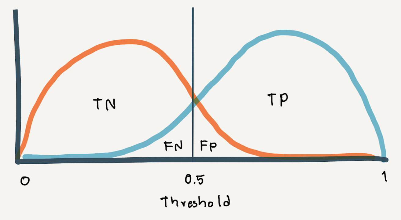
เพื่อจะลดผลการทำนายที่ทำให้เกิด False Negative สูง (เช่นในกรณีที่เราซีเรียสเรื่องการติดเชื้อ แต่ Model ทำนายผิดว่าไม่ติดเชื้อ) เราสามารถลดค่า Threshold ลง ซึ่งจะทำให้ False Positive Rate มีค่าสูงขึ้นแทน
False Positive Rate (FPR) = FP/(FP+TN)การลดค่า Threshold จะทำให้ทั้ง Recall และ False Positive Rate สูงขึ้นด้วย (Precision ต่ำ) ซึ่งจะต้องมีการ Trade-off ระหว่างประสิทธิภาพของ Model (Recall) และ False Positive Rate ที่ยอมรับได้ โดยเราจะได้เห็นความสัมพันธ์ของสองค่านี้จาก ROC Curve
ROC Curve เป็นกราฟที่แต่ละจุด (x, y) เป็นค่า False Positive Rate และ True Positive Rate (Recall) ซึ่งเกิดจากการขยับค่า Threshold ที่ต่างกัน โดยยิ่งมีการซ้อนทับของการกระจายตัวของค่าความเชื่อมั่นของทั้งสอง Class มากเท่าไหร่ เราก็จะเห็น ROC Curve มีความชันน้อยลงเท่านั้น
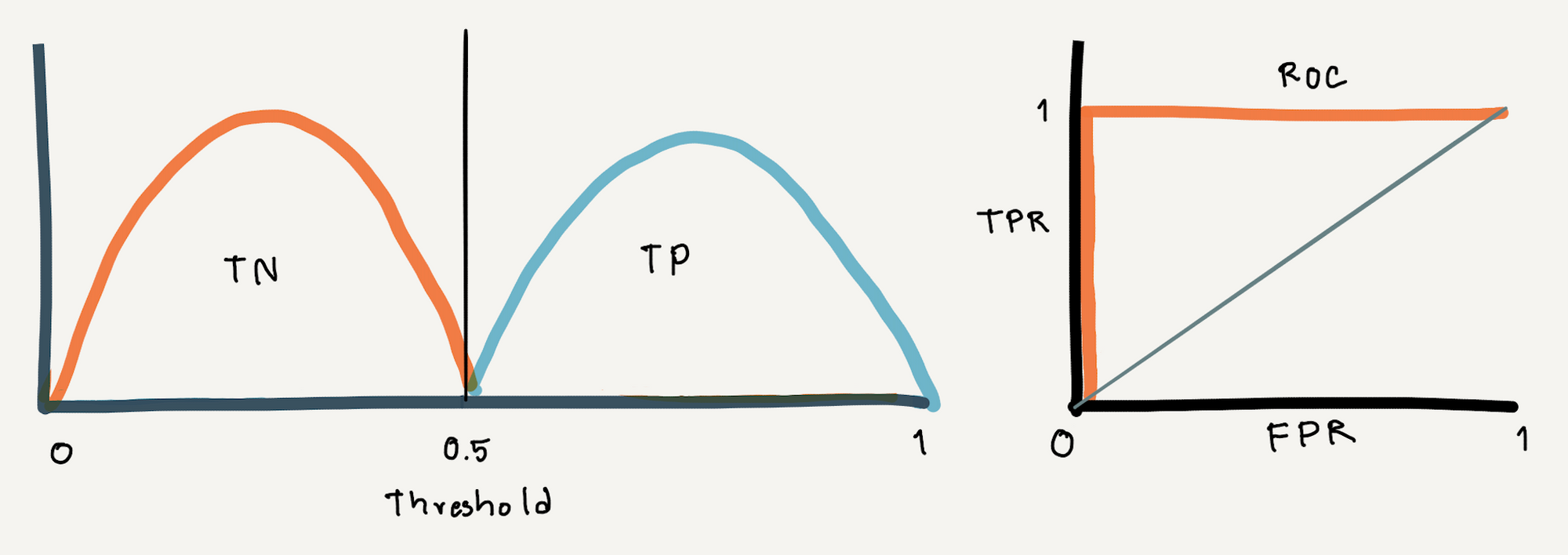
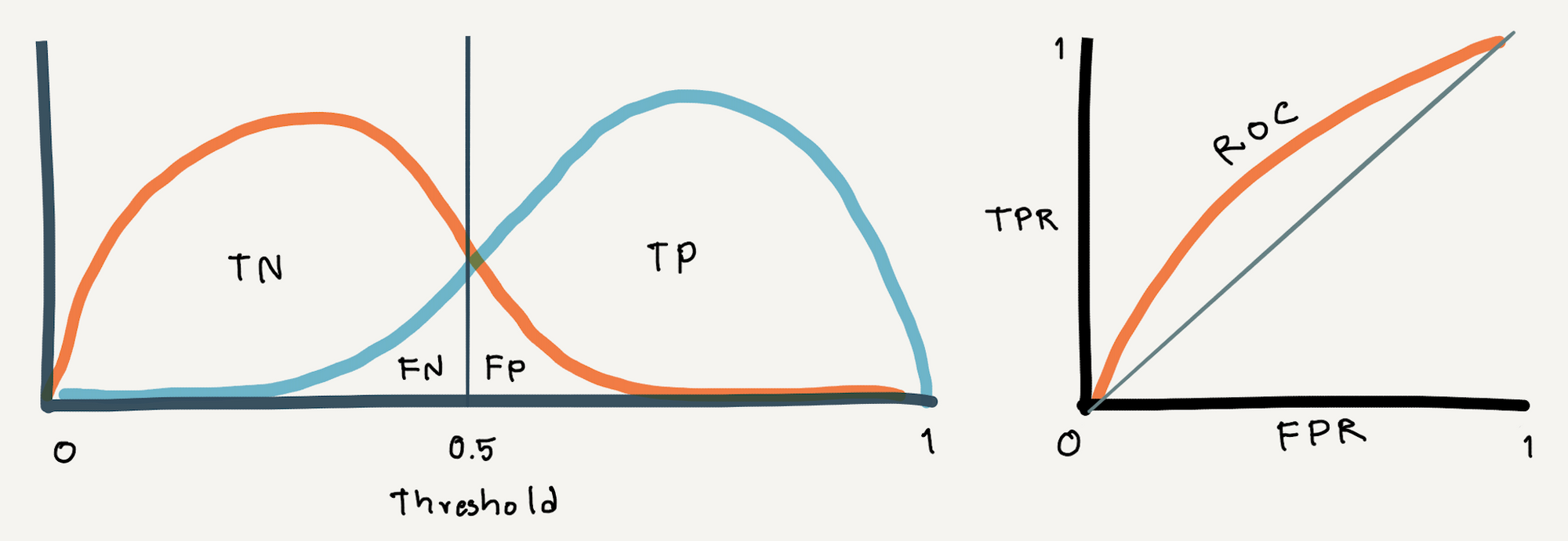
ถ้ามีการลากเส้นทะแยงมุมแบ่ง ROC Curve ออกเป็นสองส่วน ดังภาพด้านบน และกำหนดให้พื้นที่ใต้เส้นทะแยงมุมเท่ากับ 0.5 พื้นที่ใต้ ROC Curve ทั้งหมดจะมีค่าไม่เกิน 1 (100%)
ดังนั้นพื้นที่ใต้เส้นกราฟ (Area Under The Curve : AUC) จึงสามารถบอกได้ว่า Model ของเรามีความสามารถในการแยกการติดเชื้อออกจากการไม่ติดเชื้อได้ดีแค่ไหน
เราจะทดลอง Train Model แบบ Binary Classification จากข้อมูลที่ Make ขึ้นมาด้วยฟังก์ชัน make_circles ตามขั้นตอนต่อไปนี้
- Import Library ที่จำเป็นต้องใช้
import tensorflow as tf
fashion_mnist = tf.keras.datasets.fashion_mnist
to_categorical = tf.keras.utils.to_categorical

import matplotlib.pyplot as plt
from sklearn.datasets import make_circles
from sklearn.metrics import roc_curve, auc
from sklearn.model_selection import train_test_split
from sklearn.metrics import confusion_matrix
from sklearn.metrics import classification_report

import pandas as pd
import numpy as np

import plotly.express as px
import plotly
import plotly.graph_objs as go
import plotly.figure_factory as ff
import seaborn as sn

from collections import Counter- สร้าง Dataset แบบ 2 Class โดยใช้ Function make_circles ของ Sklearn
x, y = make_circles(n_samples=5000, noise=0.1, random_state=1)- แบ่งข้อมูลสำหรับ Train และ Validate โดยการสุ่มในสัดส่วน 50:50
x_train, x_val, y_train, y_val = train_test_split(x, y, test_size=0.5, shuffle= True)

x_train.shape, x_val.shape, y_train.shape, y_val.shape
((2500, 2), (2500, 2), (2500,), (2500,))
- นำ Dataset ส่วนที่ Train มาแปลงเป็น DataFrame โดยเปลี่ยนชนิดข้อมูลใน Column "class" เป็น String เพื่อทำให้สามารถแสดงสีแบบไม่ต่อเนื่องได้ แล้วนำไป Plot
x_train_pd = pd.DataFrame(x_train, columns=['x', 'y'])
y_train_pd = pd.DataFrame(y_train, columns=['class'], dtype='str')

df = pd.concat([x_train_pd, y_train_pd], axis=1)
fig = px.scatter(df, x="x", y="y", color="class")
fig.show()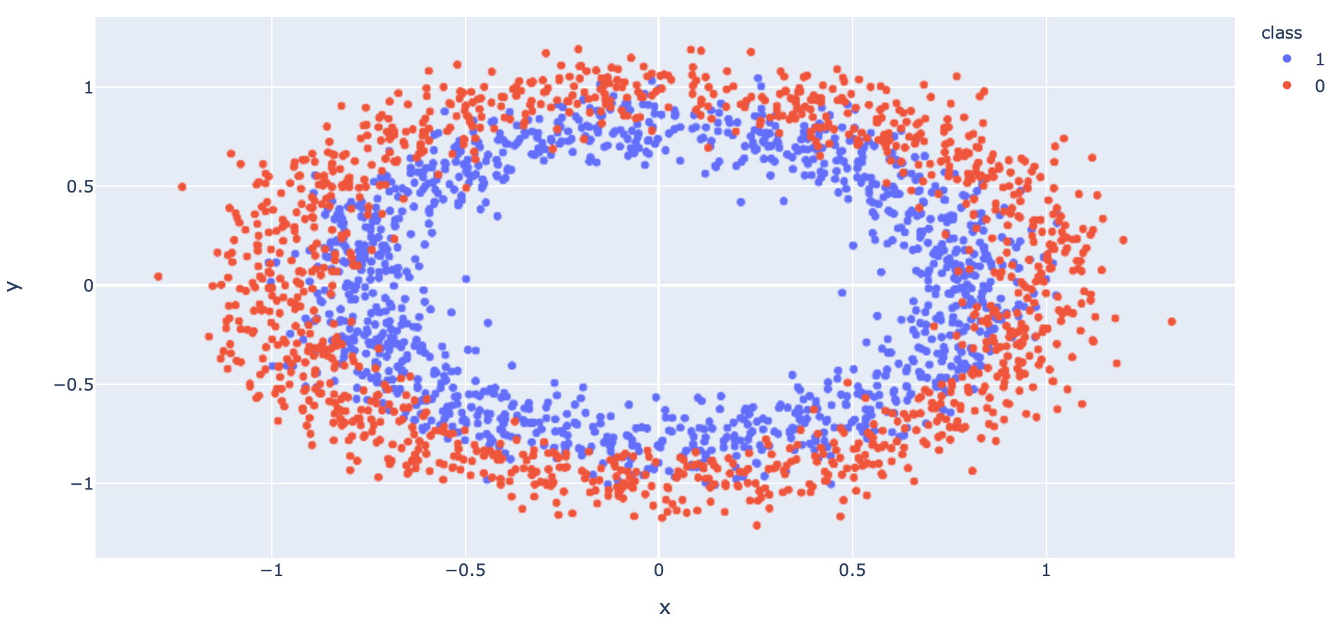
- นิยาม Model โดยกำหนด Activation Function ใน Layer สุดท้ายเป็น sigmoid
model = tf.keras.models.Sequential()
model.add(tf.keras.layers.Dense(60, input_dim=2, activation='relu', kernel_initializer='he_uniform'))
model.add(tf.keras.layers.Dropout(0.2))
model.add(tf.keras.layers.Dense(1, activation='sigmoid'))- Compile Model โดยกำหนด Loss Function เป็น binary_crossentropy
opt = tf.keras.optimizers.SGD(learning_rate=0.01, momentum=0.9)
model.compile(loss='binary_crossentropy', optimizer=opt, metrics=['accuracy'])- Train Model และประเมิน Model ในแต่ละ Epoch ด้วย Validation Dataset
his = model.fit(x_train, y_train, validation_data=(x_val, y_val), epochs=2000, verbose=1, batch_size = 256)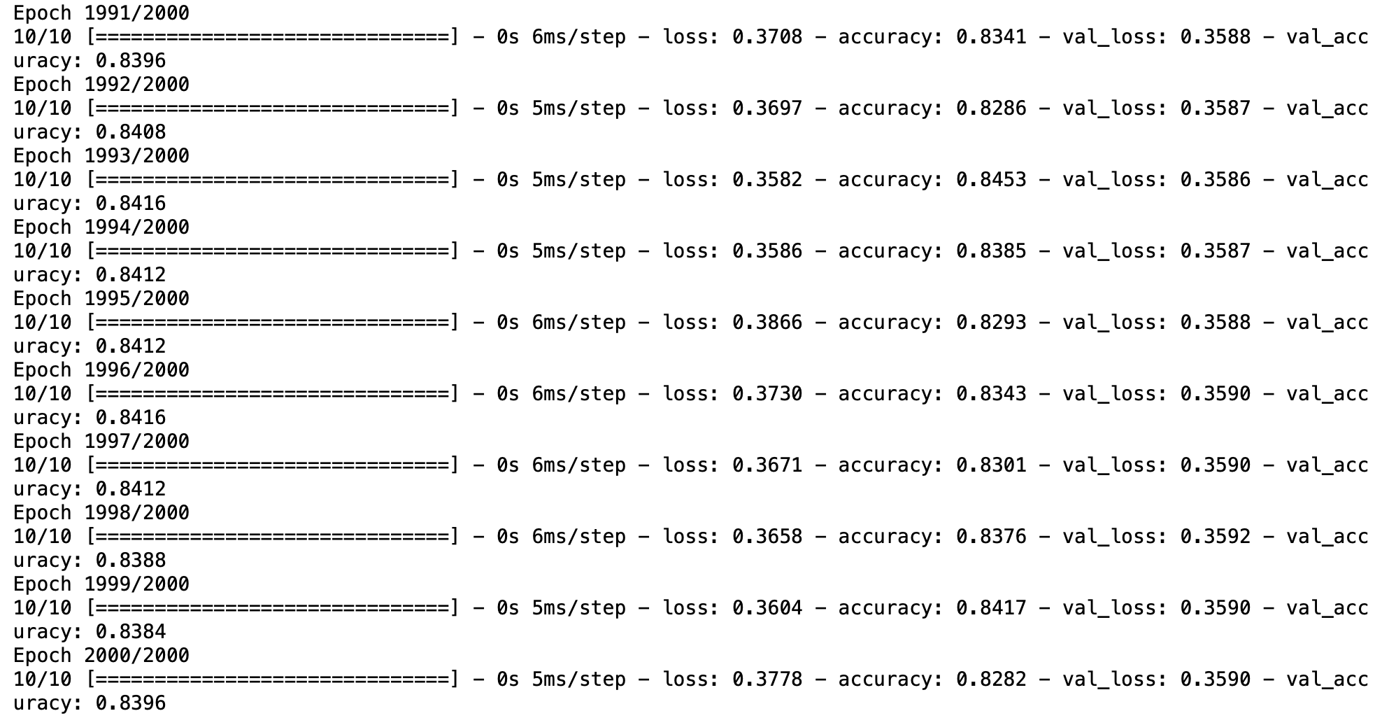
- Plot Loss
h1 = go.Scatter(y=his.history['loss'],
                    mode="lines",
                    line=dict(
                        width=2,
                        color='blue'),
                        name="loss"
                   )
h2 = go.Scatter(y=his.history['val_loss'],
                    mode="lines",
                    line=dict(
                        width=2,
                        color='red'),
                        name="val_loss"
                   )

data = [h1,h2]
layout1 = go.Layout(title='Loss',
                   xaxis=dict(title='epochs'),
                   yaxis=dict(title=''))
fig1 = go.Figure(data = data, layout=layout1)
plotly.offline.iplot(fig1)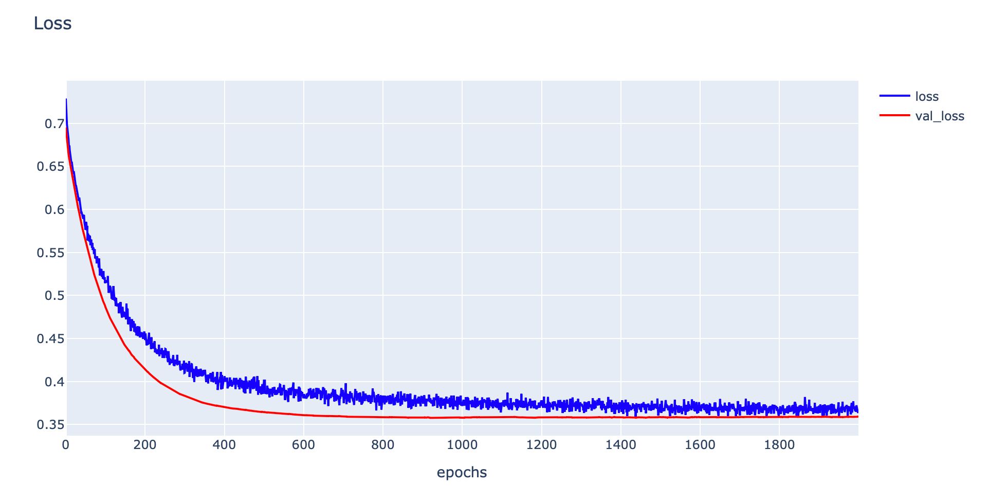
- Plot Accuracy
h1 = go.Scatter(y=his.history['accuracy'],
                    mode="lines", line=dict(
                    width=2,
                    color='blue'),
                    name="acc"
                   )
h2 = go.Scatter(y=his.history['val_accuracy'],
                    mode="lines", line=dict(
                    width=2,
                    color='red'),
                    name="val_acc"
                   )

data = [h1,h2]
layout1 = go.Layout(title='Accuracy',
                   xaxis=dict(title='epochs'),
                   yaxis=dict(title=''))
fig1 = go.Figure(data = data, layout=layout1)
plotly.offline.iplot(fig1)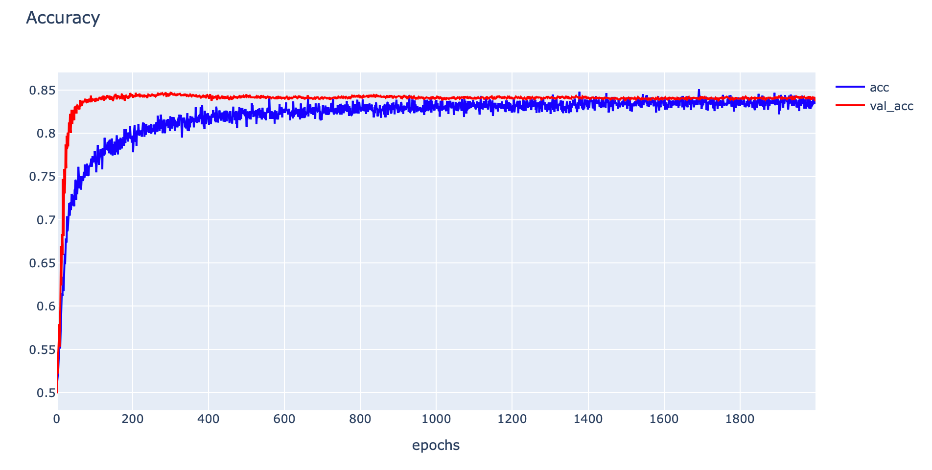
- Evaluate Model ด้วย Accuracy ของ Training Dataset และ Validation Dataset
_, train_acc = model.evaluate(x_train, y_train, verbose=0)
_, val_acc = model.evaluate(x_val, y_val, verbose=0)
print('Train: %.4f, Validation: %.4f' % (train_acc, val_acc))
Train: 0.8512, Validation: 0.8396
- ก่อนจะแสดง Confusion Matrix เราจะทดลองนับจำนวนข้อมูลในแต่ละ Class ด้วย Counter
c = Counter(y_val)
c
Counter({0: 1259, 1: 1241})
- กำหนดค่า Threshold เท่ากับ 0.5 และเรียกใช้ Function Predict
predicted_classes = (model.predict(x_val) > 0.5).astype("int32")[:,0]- คำนวณ Confusion Matrix จากผลเฉลย (y_val) และผลลัพธ์จากการ Predict (predicted_classes)
cm = confusion_matrix(y_val, predicted_classes)
cm
- กำหนดชื่อ Class และนิยาม cm_plot สำหรับ Plot Confusion Matrix ด้วย Plotly
labels = ['No', 'Yes']def cm_plot(cm, labels):
x = labels
y = labels
z_text = [[str(y) for y in x] for x in cm]
fig = ff.create_annotated_heatmap(cm, x=x, y=y, annotation_text=z_text, colorscale='blues')
fig.update_layout(title_text='Confusion Matrix')
fig.add_annotation(dict(font=dict(color="black",size=13),
x=0.5,
y=-0.15,
showarrow=False,
text="Predicted Value",
xref="paper",
yref="paper"
))
fig.add_annotation(dict(font=dict(color="black",size=13),
x=-0.20,
y=0.5,
showarrow=False,
text="Real Value",
textangle=-90,
xref="paper",
yref="paper"
))
fig.update_layout(margin=dict(t=50, l=200))
fig['layout']['yaxis']['autorange'] = "reversed"
fig['data'][0]['showscale'] = True
fig.show()cm_plot(cm, labels)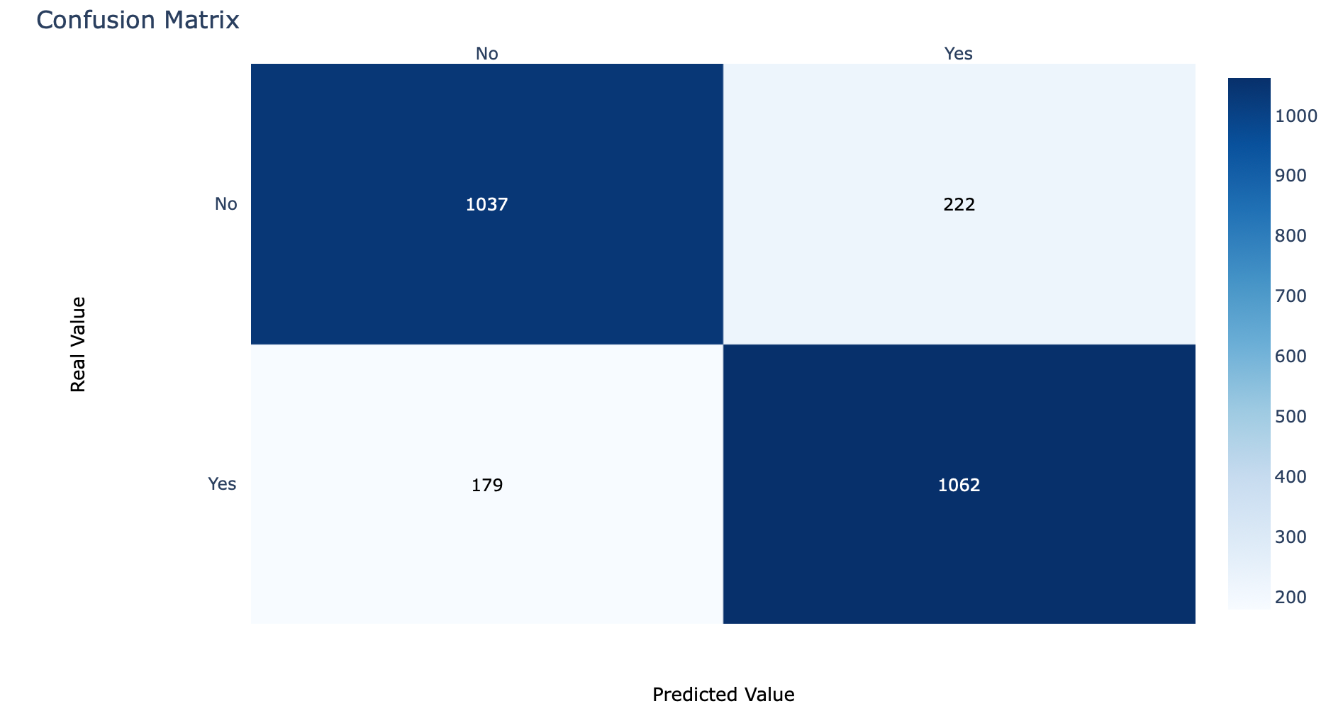
- เราสามารถแสดงค่า Precision, Recall, F1-score รวมทั้งค่าเฉลี่ยของ Precision, Recall, F1-score ทั้งแบบ Macro avg และ Weight avg ด้วย Function classification_report ซึ่งค่า Macro avg และ Weight avg สามารถคำนวณได้ดังตัวอย่างต่อไปนี้
Macro avg ของ Precision = (0.8528+0.8271)/2 = 0.83995
Weight avg ของ Precision = 0.8528*(1259/2500)+0.8271*(1241/2500) = 0.84004252
จากตัวอย่าง Macro avg และ Weight avg ของ Precision มีค่าต่างกัน เนื่องจากจำนวนข้อมูลทั้ง 2 Class ไม่เท่ากัน (Imbalanced Classes) ซึ่งเมื่อข้อมูลมีลักษณะ Imbalanced เราจะดูค่าเฉลี่ยแบบ Weight avg เป็นหลักครับ
print(classification_report(y_val, predicted_classes, target_names=labels, digits=4))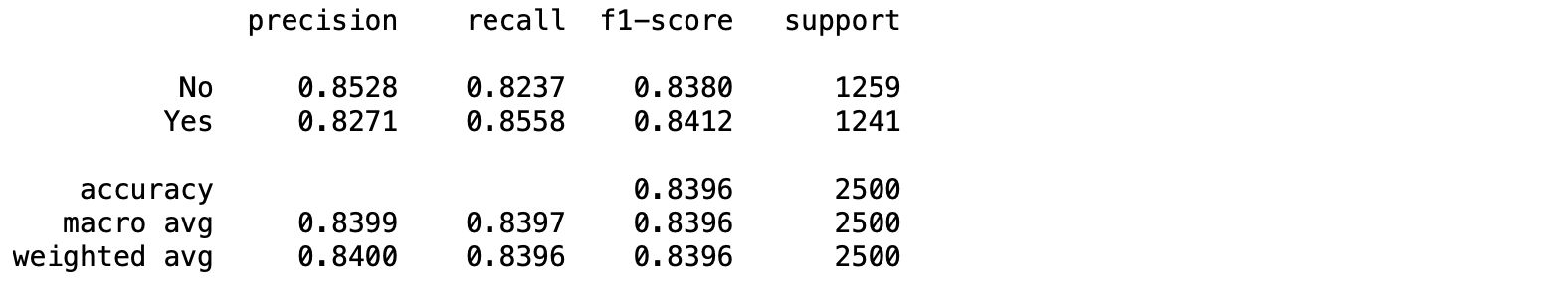
นอกจาก Precision, Recall, F1-score แล้ว classification_report ยังแสดงจำนวนข้อมูลในแต่ละ Class ด้วยค่า Support
- เพื่อจะแสดงการกระจายตัวของค่าความเชื่อมั่นที่ Model ทำนาย จาก Validation Dataset ทั้ง 2 Class เราจะนำค่าความเชื่อมั่นและ Class ของ Dataset มาสร้างเป็น DataFrame และ Plot เป็น Histogram
y_score = model.predict(x_val)
y_score = y_score[:,0]
distribution_df = pd.DataFrame(data={'Score': y_score, 'Class': y_val})
distribution_df.head()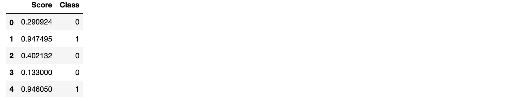
distribution_df.loc[distribution_df['Class'] == 1, 'Class'] = 'Yes'
distribution_df.loc[distribution_df['Class'] == 0, 'Class'] = 'No'
distribution_df.sample(10)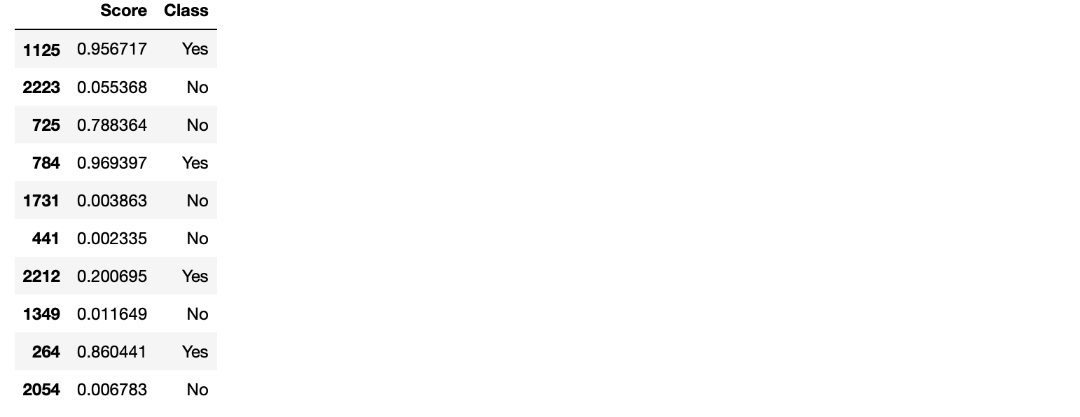
fig = px.histogram(distribution_df, x='Score', color='Class', nbins=50)
fig.update_layout(barmode='overlay')
fig.update_traces(opacity=0.85)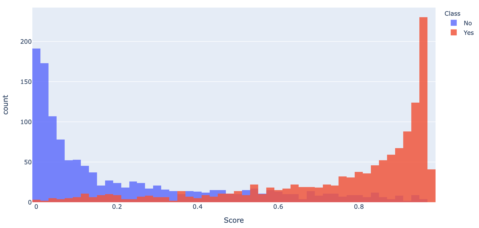
จาก Histogram พบว่ามีการซ้อนทับกันของค่าความเชื่อมั่นของทั้งสอง Class ซึ่งจะทำให้พื้นที่ใต้ ROC Curve (AUC) น้อยกว่า 1
โดยเราจะคำนวณค่า True Positive Rate และ False Positive Rate ด้วยฟังก์ชัน roc_curve และนำ True Positive Rate และ False Positive Rate ที่ได้ไปคำนวณ AUC อีกทีด้วยฟังก์ชัน auc
fpr, tpr, threshold = roc_curve(y_val, y_score)
roc_auc = auc(fpr, tpr)
roc_df = pd.DataFrame(data={'False Positive Rate': fpr, 'True Positive Rate': tpr, 'Threshold': threshold})
roc_df.head()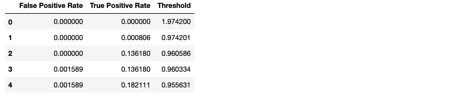
def binary_roc_plot(roc_df, roc_auc):
    fig = px.area(
        data_frame=roc_df,
        x='False Positive Rate',
        y='True Positive Rate',
        hover_data=['Threshold'],
        title=f'ROC Curve (AUC={roc_auc:.4f})',
        width=700, height=500,
    )

    fig.add_shape(
        type='line', line=dict(dash='dash'),
        x0=0, x1=1, y0=0, y1=1
    )

    hovertemplate = 'False Positive Rate=%{x:.4f}<br>True Positive Rate=%{y:.4f}<br>Threshold=%{customdata[0]:.4f}'
    fig.update_traces(hovertemplate=hovertemplate)

fig.show()- Plot ROC Curve และ AUC
binary_roc_plot(roc_df, roc_auc)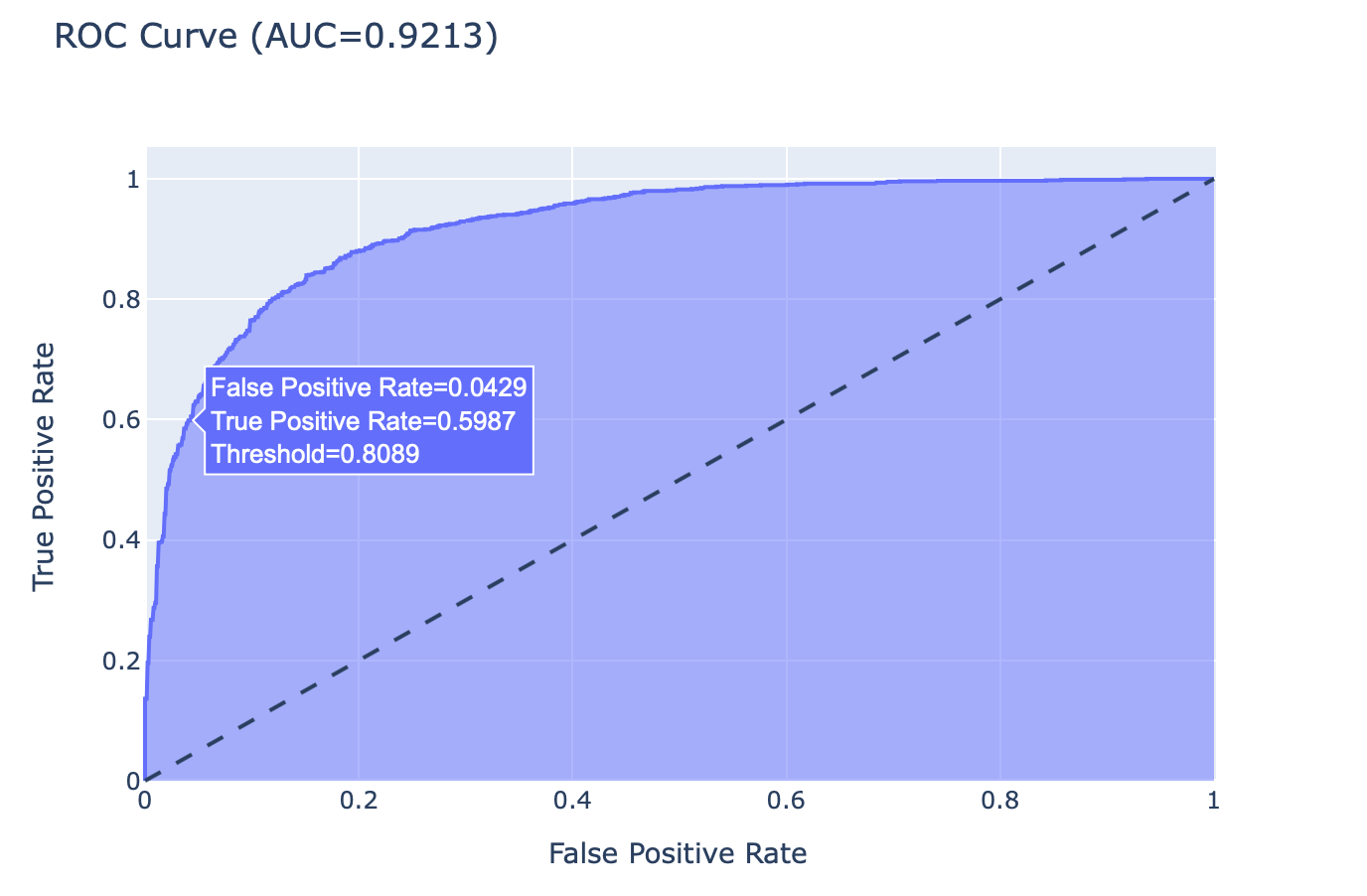
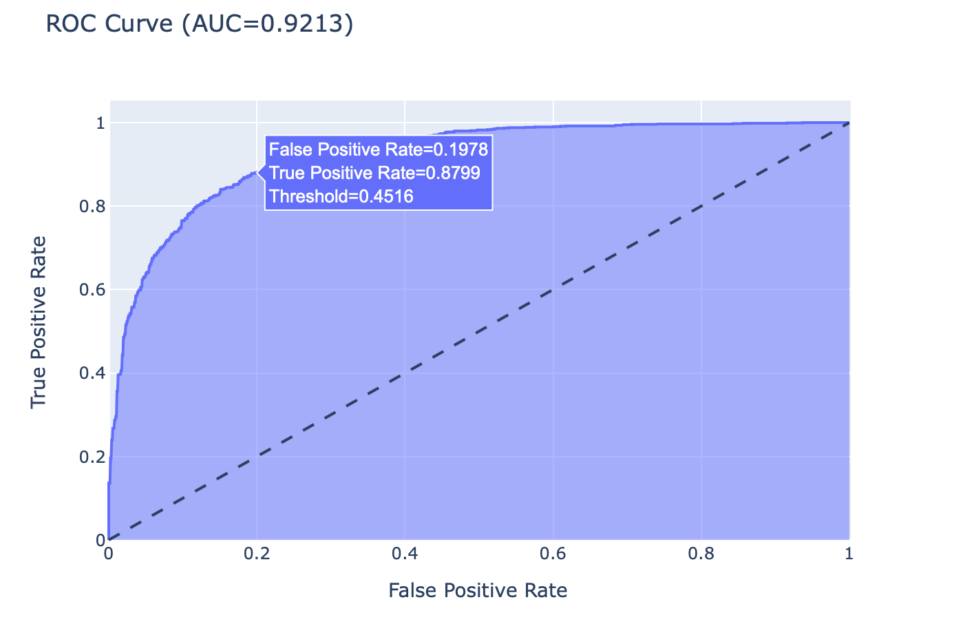
เมื่อมีการเลื่อน Mouse ไปยังจุดต่างๆ บน ROC Curve จากซ้ายไปขวา เราจะเห็นค่า Threshold ค่อยๆ ลดลง ขณะที่ค่า True Positive Rate (Recall) และ False Positive Rate เพิ่มขึ้น ซึ่งในกรณีของ Model ที่มีการทำนายการติดเชื้อไวรัส โคโรนา จากภาพ X-ray ปอด การพิจารณาว่าจะลดค่า Threshold หรือไม่อย่างไร จะขึ้นอยู่กับว่าเราจะยอมให้เกิดการทำนายผิดว่าติดเชื้อ ทั้งๆ ที่ไม่ติดมากน้อยแค่ไหน
- เราจะทดลองกำหนดค่า Threshold เท่ากับ 0.4516 และเรียกใช้ Function Predict
predicted_classes = (model.predict(x_val) > 0.4516).astype("int32")[:,0]- คำนวณ Confusion Matrix ใหม่ จากผลเฉลยและผลลัพธ์จากการ Predict
cm = confusion_matrix(y_val, predicted_classes)
cm
- Plot Confusion Matrix ด้วย Plotly
cm_plot(cm, labels)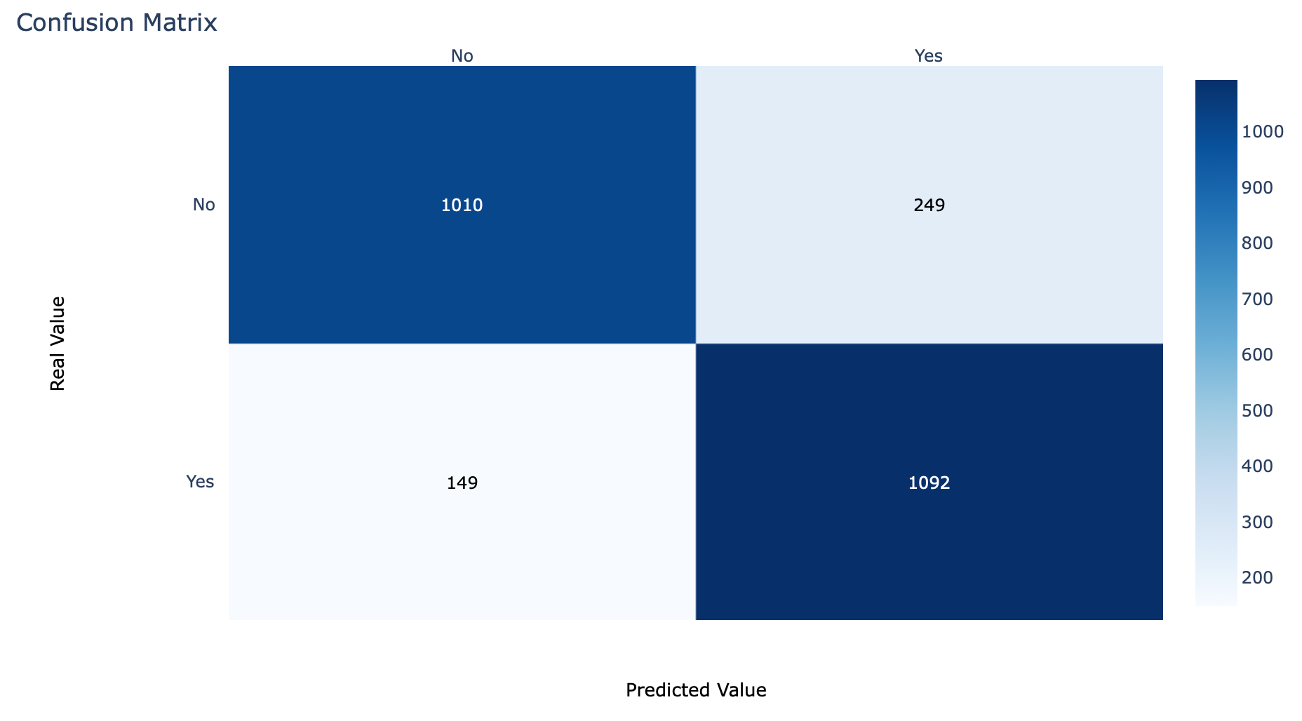
- แสดง Precision, Recall, F1-score ด้วย classification_report
print(classification_report(y_val, predicted_classes, target_names=labels, digits=4))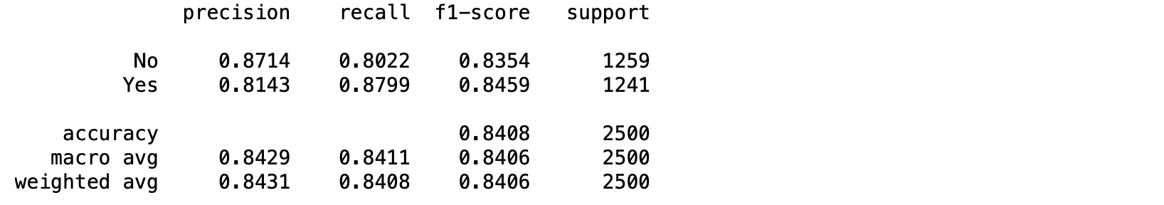
เมื่อมีการลดค่า Threshold จาก 0.5 เป็น 0.4516 ค่า Recall ของ Class 1 จะเพิ่มขึ้นจาก 0.8558 เป็น 0.8799
Multi-Class Classification Evaluation
Multi-Class Classification เป็น Model ที่มีการกำหนด Label หรือ Class มากกว่า 2 Class ผลลัพธ์ของ Model จะบอกถึงค่าความเชื่อมั่นในการทำนายของแต่ละ Class โดยค่าความเชื่อมั่นของทุกๆ Class รวมกันจะเท่ากับ 1.0
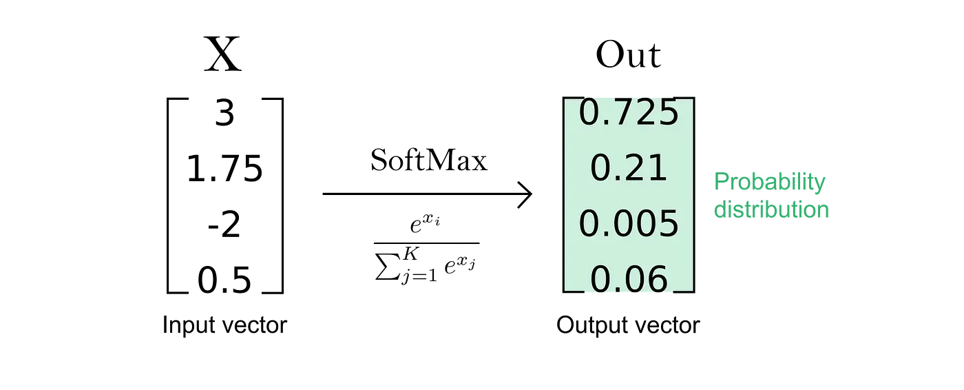
เพื่อจะทำให้ Model ทำนายผลออกมาเป็นค่าความเชื่อมั่นที่ทุก Class รวมกันเท่ากับ 1.0 เราจะต้องคอนฟิก Activate Function ใน Output Layer เป็น Softmax แทน Sigmoid โดย Class ที่ถูกทำนาย จะถูกเลือกมาจากตำแหน่งของค่าความเชื่อมั่นที่มากที่สุด แทนที่จะเป็นการพิจารณาจากค่า Threshold
เราจะทดลอง Train Model แบบ Multi-Class Classification จาก Fashion MNIST Dataset ตามขั้นตอนต่อไปนี้
- กำหนดค่าตัวแปรต่างๆ
IMG_ROWS = 28
IMG_COLS = 28
NUM_CLASSES = 10
VAL_SIZE = 0.2
RANDOM_STATE = 99
BATCH_SIZE = 256

INPUT_SHAPE = (IMG_ROWS, IMG_COLS, 1)- Load Fashion MNIST Dataset
(x_train, y_train), (x_test, y_test) = fashion_mnist.load_data()

print("Fashion MNIST train -  rows:",x_train.shape[0]," columns:", x_train.shape[1], " rows:", x_train.shape[2])
print("Fashion MNIST test -  rows:",x_test.shape[0]," columns:", x_test.shape[1], " rows:", x_test.shape[2])
Fashion MNIST train - rows: 60000 columns: 28 rows: 28
Fashion MNIST test - rows: 10000 columns: 28 rows: 28
- กำหนดชื่อในแต่ละ Class แล้ว Plot ภาพทั้งหมด 16 ภาพ
labels = ['T-shirt/top', 'Trouser', 'Pullover', 'Dress', 'Coat', 'Sandal', 'Shirt', 'Sneaker', 'Bag', 'Ankle boot']for i in range(16):
ax = plt.subplot(4, 4, 1+i)
ax.set_xticks([])
ax.set_yticks([])
ax.set_title('%s'%(labels[y_train[i]]))
plt.imshow(x_train[i], cmap=plt.get_cmap('Blues'))
plt.tight_layout()
plt.savefig('fashion_mnist.jpeg', dpi=300)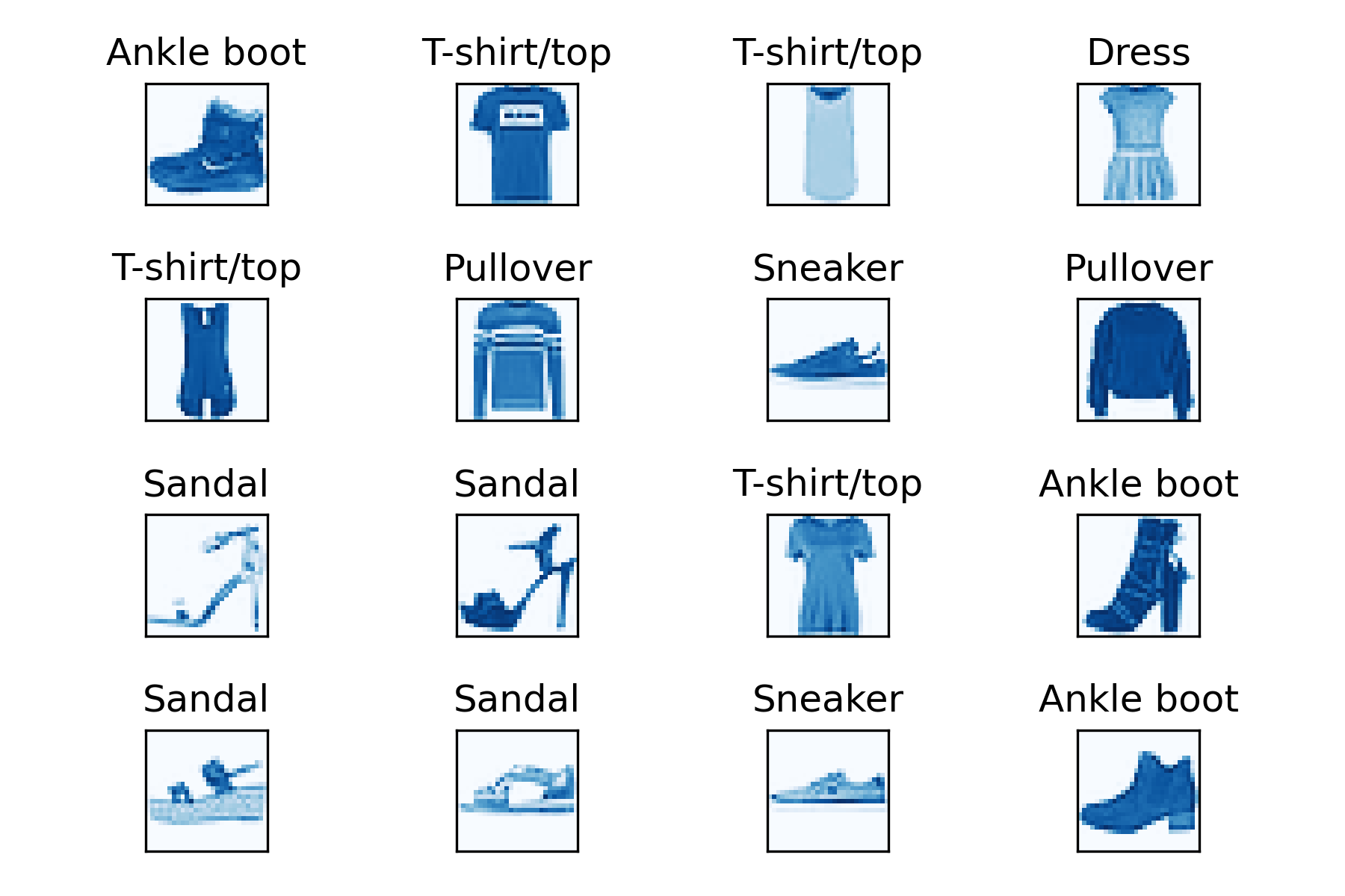
- ขยายมิติของข้อมูล เพื่อเตรียมนำเข้าไป Train ใน Model
print(x_train.shape, x_test.shape)

x_train = x_train.reshape((x_train.shape[0], 28, 28, 1))
x_test = x_test.reshape((x_test.shape[0], 28, 28, 1))

print(x_train.shape, x_test.shape)
(60000, 28, 28) (10000, 28, 28)
(60000, 28, 28, 1) (10000, 28, 28, 1)
- ทำ Scaling
x_train = x_train / 255.0
x_test = x_test / 255.0- เข้ารหัสผลเฉลยแบบ One-hot Encoding
y_train = to_categorical(y_train, NUM_CLASSES)
y_test = to_categorical(y_test, NUM_CLASSES)- แบ่งข้อมูลสำหรับ Train และ Validation โดยการสุ่มในสัดส่วน 80:20
x_train, x_val, y_train, y_val = train_test_split(x_train, y_train, test_size=VAL_SIZE, random_state=RANDOM_STATE)

x_train.shape, x_val.shape, y_train.shape, y_val.shape
((48000, 28, 28, 1), (12000, 28, 28, 1), (48000, 10), (12000, 10))
- นิยาม Model
#Feature Extraction
model = tf.keras.Sequential()
model.add(tf.keras.layers.Conv2D(32, kernel_size=(3, 3), activation='relu', input_shape=INPUT_SHAPE))
model.add(tf.keras.layers.Conv2D(64, (3, 3), activation='relu'))
model.add(tf.keras.layers.MaxPooling2D(pool_size=(2, 2)))
model.add(tf.keras.layers.Dropout(0.25))

#Image Classification
model.add(tf.keras.layers.Flatten())
model.add(tf.keras.layers.Dense(128, activation='relu'))
model.add(tf.keras.layers.Dropout(0.5))
model.add(tf.keras.layers.Dense(NUM_CLASSES, activation='softmax'))- Compile Model
optimizer = tf.keras.optimizers.Adam()
model.compile(optimizer = optimizer, loss = "categorical_crossentropy", metrics=["accuracy"])

model.summary()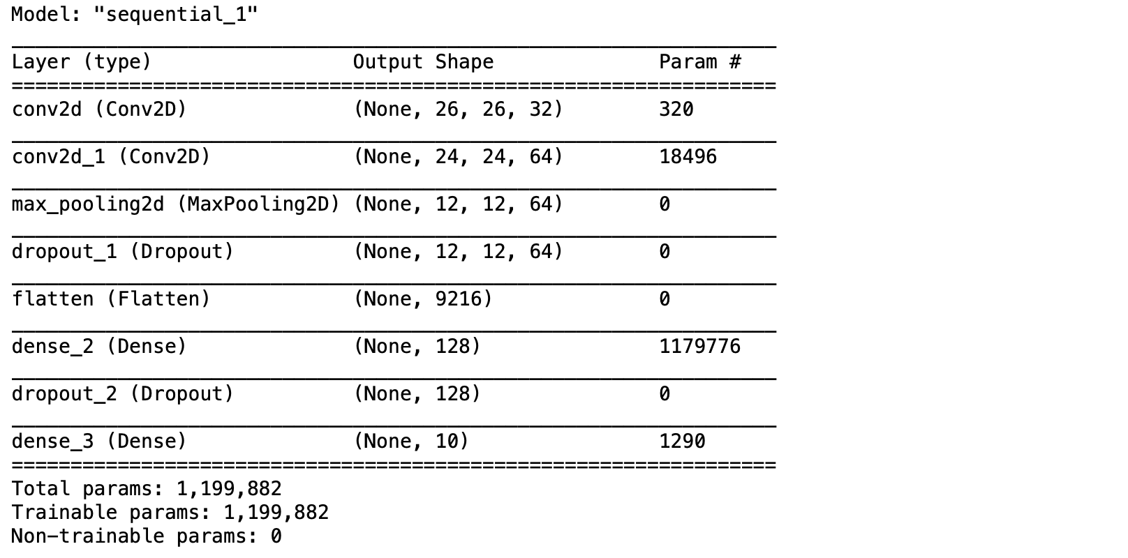
- Train Model
NO_EPOCHS = 15

history = model.fit(x_train, y_train,
                  batch_size=BATCH_SIZE,
                  epochs=NO_EPOCHS,
                  verbose=1,
                  validation_data=(x_val, y_val))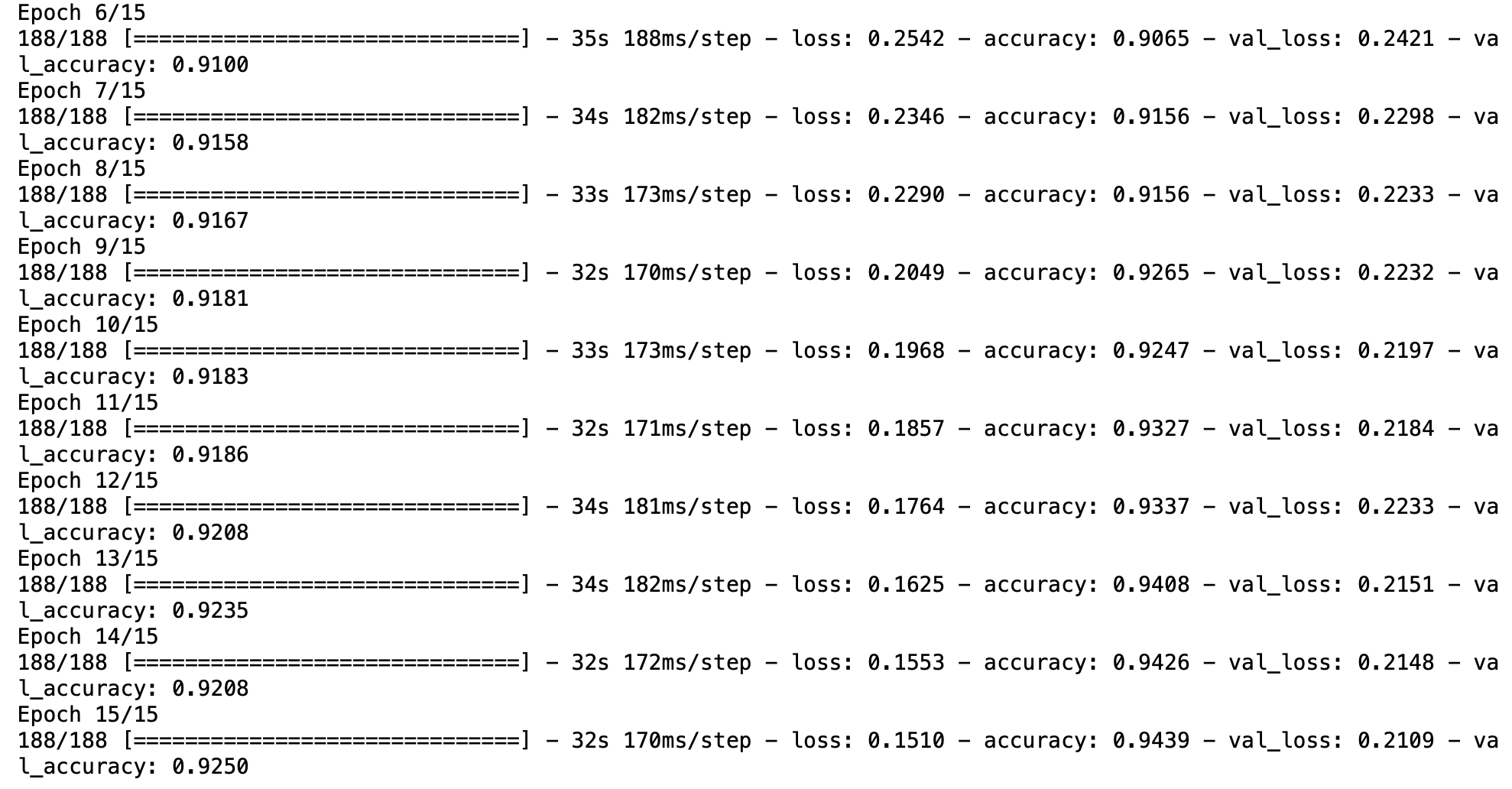
- Plot Loss
h1 = go.Scatter(y=history.history['loss'],
                    mode="lines",
                    line=dict(
                        width=2,
                        color='blue'),
                        name="loss"
                   )
h2 = go.Scatter(y=history.history['val_loss'],
                    mode="lines",
                    line=dict(
                        width=2,
                        color='red'),
                        name="val_loss"
                   )

data = [h1,h2]
layout1 = go.Layout(title='Loss',
                   xaxis=dict(title='epochs'),
                   yaxis=dict(title=''))
fig1 = go.Figure(data = data, layout=layout1)
plotly.offline.iplot(fig1)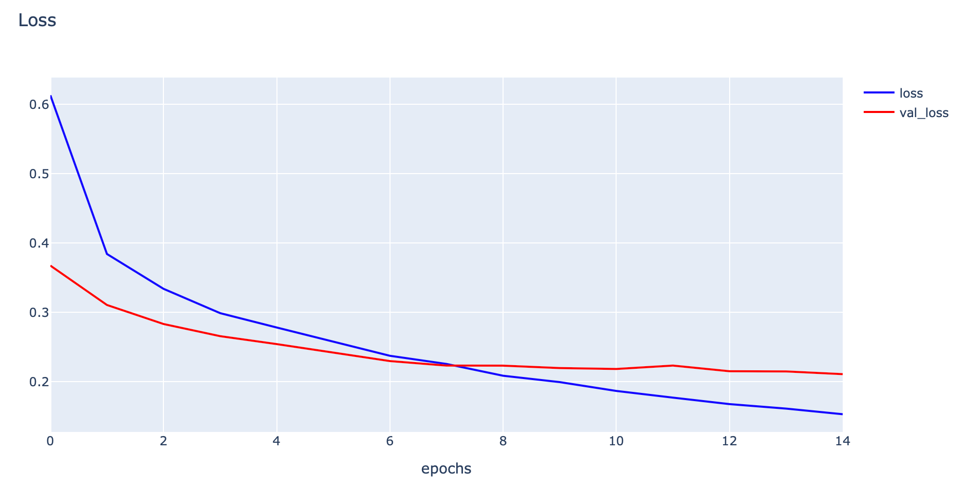
- Plot Accuracy
h1 = go.Scatter(y=history.history['accuracy'],
                    mode="lines",
                    line=dict(
                        width=2,
                        color='blue'),
                        name="acc"
                   )
h2 = go.Scatter(y=history.history['val_accuracy'],
                    mode="lines",
                    line=dict(
                        width=2,
                        color='red'),
                        name="val_acc"
                   )

data = [h1,h2]
layout1 = go.Layout(title='Accuracy',
                   xaxis=dict(title='epochs'),
                   yaxis=dict(title=''))
fig1 = go.Figure(data = data, layout=layout1)
plotly.offline.iplot(fig1)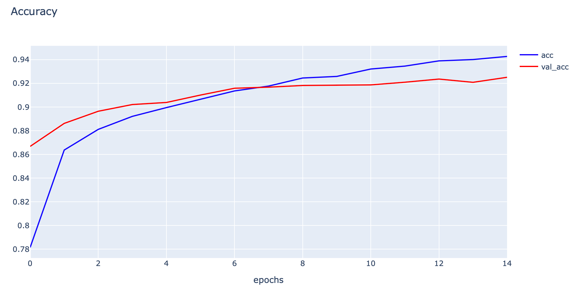
- Predict ภาพจาก Testing Dataset แล้วแปลงค่าความมั่นใจเป็นหมายเลขของ Class
predicted_classes = model.predict(x_test)
predicted_classes = np.argmax(predicted_classes, axis=1)- แปลงผลเฉลยที่มีการเข้ารหัสแบบ One-hot Encoding เป็นหมายเลขของ Class เพื่อใช้ในการสร้าง Confusion Matrix
y_true = np.argmax(y_test, axis=1)- ก่อนจะแสดง Confusion Matrix ทดลองนับจำนวนข้อมูลในแต่ละ Class ด้วย Counter
c = Counter(y_true)
c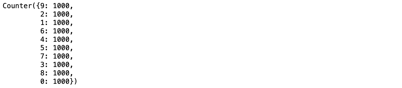
- คำนวณ Confusion Matrix จากผลเฉลย และผลลัพธ์จากการ Predict
cm = confusion_matrix(y_true, predicted_classes)
cm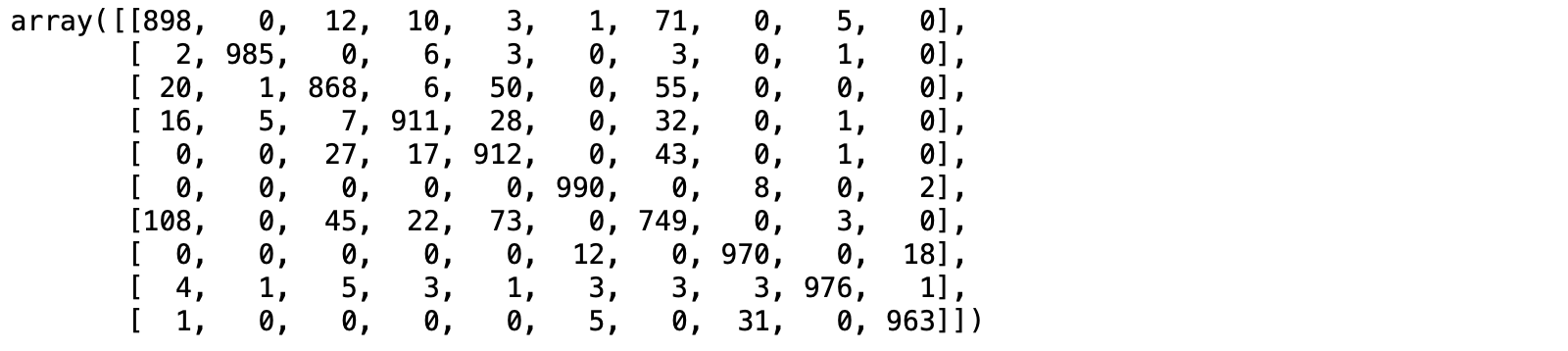
- Plot Confusion Matrix ด้วย Plotly
cm_plot(cm, labels)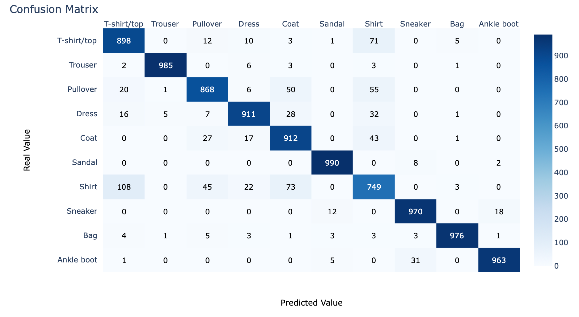
- แสดง Precision, Recall, F1-score ด้วย classification_report
print(classification_report(y_true, predicted_classes, target_names=labels, digits=4))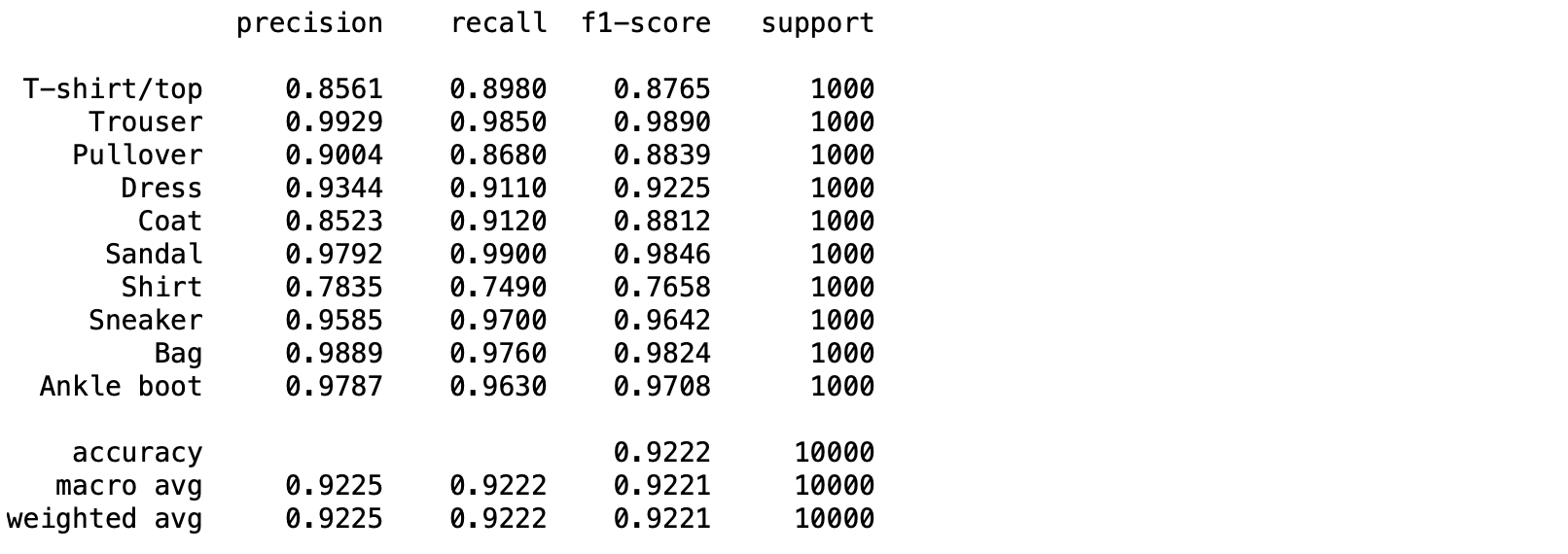
- เราจะ Plot AUC Curve และคำนวณ ROC ของภาพแต่ละ Class ในทำนองเดียวกับ Binary Classification Model ดังนั้นจึงต้องใช้ค่าความเชื่อมั่นในแต่ละ Class ในการคำนวณ True Positive Rate และ False Positive Rate
predicted_score = model.predict(x_test)
predicted_score.shape, y_test.shape
((10000, 10), (10000, 10))
- Plot ROC Curve และ AUC รวมกันในที่เดียวทั้งหมด 10 Class
hovertemplate = 'False Positive Rate=%{x:.4f}<br>True Positive Rate=%{y:.4f}<br>Threshold=%{text:.4f}'
fig = go.Figure()
fig.add_shape(
    type='line', line=dict(dash='dash'),
    x0=0, x1=1, y0=0, y1=1
)

for i in range(predicted_score.shape[1]):
    y_real = y_test[:, i]
    y_score = predicted_score[:, i]

    fpr, tpr, threshold = roc_curve(y_real, y_score)
    auc_score = auc(fpr, tpr)

    name = f"{labels[i]}, AUC={auc_score:.4f}"
    fig.add_trace(go.Scatter(x=fpr, y=tpr, name=name, mode='lines', text=threshold, hovertemplate=hovertemplate))

fig.update_layout(
    title='ROC Curve and AUC',
    xaxis_title='False Positive Rate',
    yaxis_title='True Positive Rate',
)

fig.show()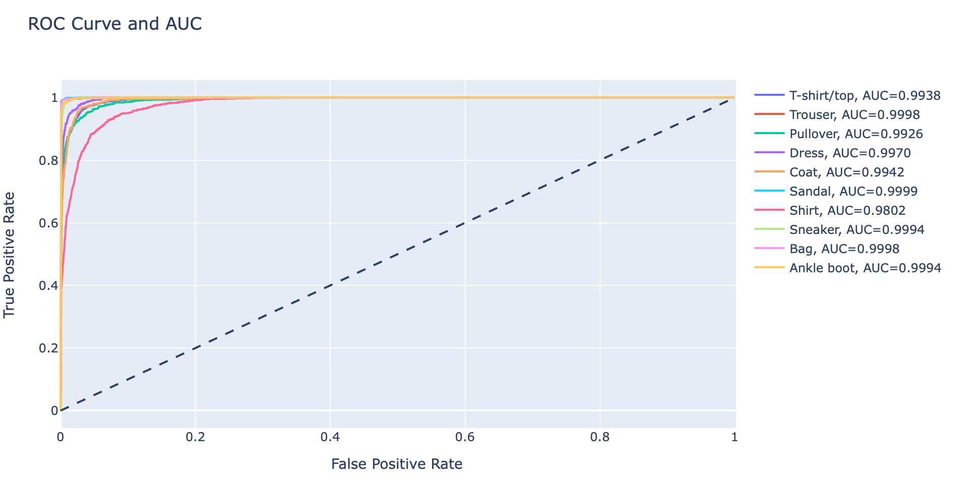
จะเห็นว่า Class 6 (Shirt) มีค่า ROC น้อยกว่า Class อื่นๆ อย่างเห็นได้ชัด ซึ่งแสดงว่า Model มีความสามารถในการแยกภาพ Class 6 ออกจาก Class อื่นๆ ได้ไม่ดีนัก ดังนั้นเราจะกรองภาพเฉพาะ Class นี้ ที่ทำนายผิด มา Plot เพื่อทำความเข้าใจ Dataset ด้วยคำสั่งต่อไปนี้
y_true, predicted_classes
false_predict = y_true!=predicted_classes

class6 = y_true==6

false_predict_class6 = class6 & false_predict

Counter(false_predict_class6)
Counter({False: 9749, True: 251})
class6_img = x_test[false_predict_class6]
class6_y = predicted_classes[false_predict_class6]
false_predict_labels = [labels[class_num] for class_num in class6_y]
for i in range(16):
ax = plt.subplot(4, 4, 1+i)
ax.set_xticks([])
ax.set_yticks([])
ax.set_title('%s'%(false_predict_labels[i]), color='red')
plt.imshow(class6_img[i], cmap=plt.get_cmap('Blues'))
plt.tight_layout()
plt.savefig('class6_fashion_mnist.jpeg', dpi=300)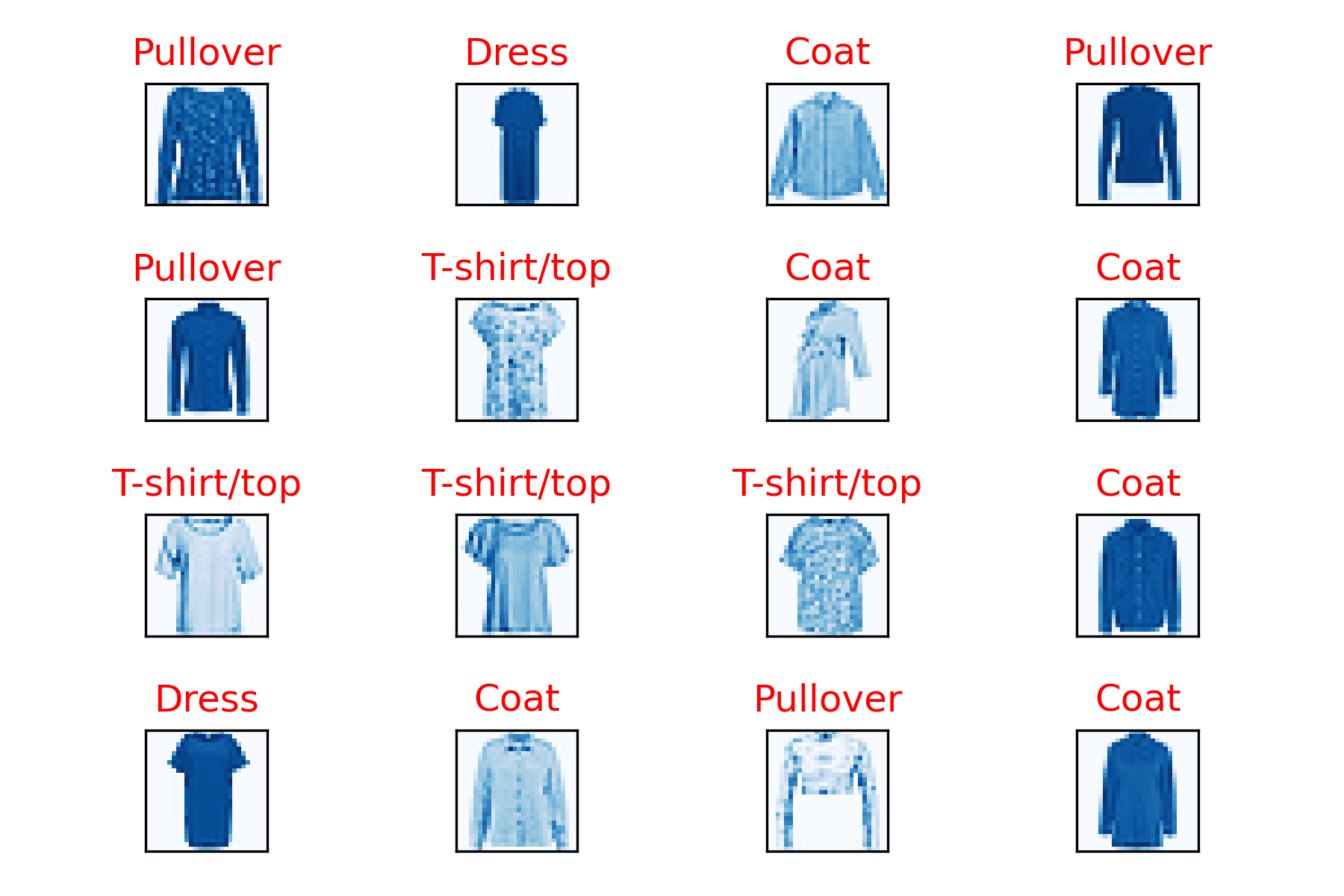
จากภาพ Class 6 (Shirt) ของ Test Dataset พบว่า Model ทำนายผิดเป็น Class ต่างๆ ได้แก่ Pullover, Dress และ Coat ฯลฯ ซึ่งดูเหมือนว่าบางภาพใน Fashion MNIST Dataset ถูก Label ยังไม่ถูกต้อง ดังเช่นภาพที่ 2 ที่ควร Label เป็น Dress มากกว่า Shirt
ซึ่งถ้าหากพบว่ามีการ Label ไม่ถูกต้องเป็นจำนวนมาก เราอาจต้องกลับไปแก้ไขการ Label Dataset (Train/Validate/Test) เสียก่อน แล้วค่อยกลับมา Train Model ใหม่อีกครั้งครับ