Sentiment Analysis using CNN

บทความโดย อ.ดร.ณัฐโชติ พรหมฤทธิ์และอ.ดร.สัจจาภรณ์ ไวจรรยา
ภาควิชาคอมพิวเตอร์
คณะวิทยาศาสตร์
มหาวิทยาลัยศิลปากร

จาก Workshop ที่แล้ว เราได้ทดลองสร้าง Model เพื่อทำ Sentiment Analysis โดยใช้ Deep Learning Model แบบ RNN ทั้งแบบ LSTM และ GRU กับชุดข้อมูลความคิดเห็นที่มีต่อสินค้า และบริการ ซึ่งรวบรวมโดย Wisesight (Thailand) Co., Ltd.

ใน Workshop นี้ เราจะใช้ชุดข้อมูลเดิมในการทำ Sentiment Analysis Model แต่เปลี่ยนวิธีการสร้าง Model ใหม่ โดยใช้เทคนิคที่เรียกว่า Convolutional Neural Network (CNN) ซึ่งเป็น Neural Network ที่นิยมใช้กันมากในงานด้าน Classification

Convolutional Neural Network (CNN)

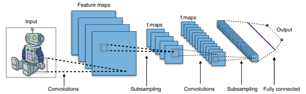
https://commons.wikimedia.org/wiki/File:Typical_cnn.png

Convolutional Neural Network (CNN) เป็น Neural Network ที่มอง Dataset ที่รับผ่าน Input Layer เป็นเหมือนภาพภาพหนึ่ง เช่นเดียวกับที่จอประสาทตาของมนุษย์มีการรับแสงที่ตกกระทบมาจากวัตถุต่างๆ

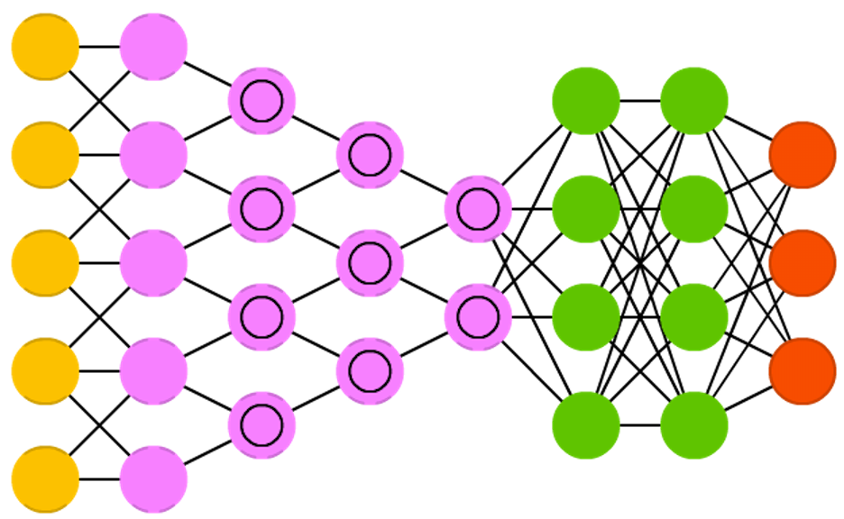
ภาพจาก http://primo.ai/index.php?title=(Deep)_Convolutional_Neural_Network_(DCNN/CNN)

จากภาพ CNN ด้านบน จะมี Input Node สำหรับรับข้อมูล และ Output Node สำหรับคำนวณผลลัพธ์ รวมทั้ง Hidden Layer อีก 6 Layer ดังนั้นจึงมีจำนวน Layer ทั้งหมด 7 Layer ไม่รวม Input Layer โดยเราจะเรียก Neural Network ที่มีจำนวน Hidden Layer มากๆ ว่า Deep Neural Network หรือ Deep Learning ซึ่งโดยปกติถ้ามันมี Hidden Layer ตั้งแต่ 3 Layer ขึ้นไป เราจะเริ่มเรียกมันว่า Deep Learning

CNN มมักจะถูกนำไปใช้กับงานที่มีลักษณะเป็นข้อมูล 2 มิติ เช่นงานด้านภาพ ซึ่ง Pixel ของ ภาพ จะมีความสัมพันธ์กันในเชิงพื้นที่ (Spatial Relationship) ดังนั้นเมื่อเรานำ CNN มาใช้กับข้อมูลประเภทข้อความ เราจะต้องแปลงข้อมูลที่เป็นข้อความให้มีลักษณะเป็นภาพด้วย

ตัวอย่างการใช้ CNN กับงานด้าน Text

ก่อนที่เราจะเริ่มลงมือ Workshop กัน ขอยกตัวอย่างภาพโครงสร้างของ Model แบบ CNN นำไปใช้กับงานด้านข้อความ

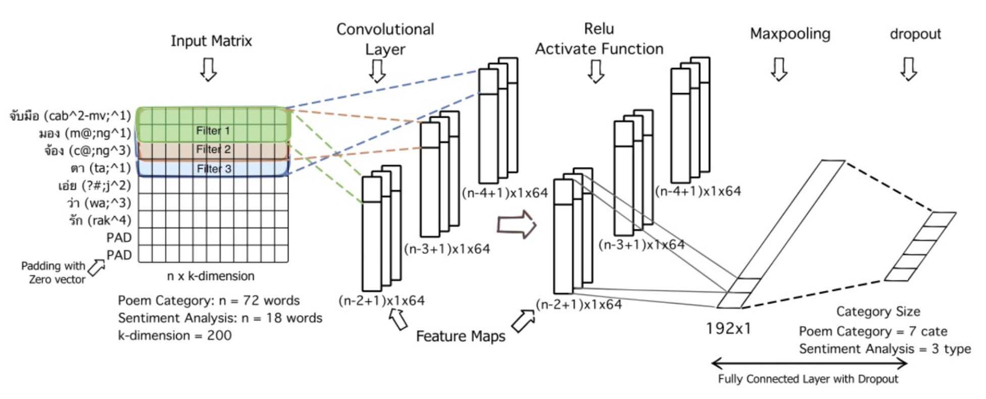
จากภาพด้านบน แทนโมเดล 2 โมเดล คือ 1) จำแนกประเภทกลอน และ 2) จำแนกทัศนคติในกลอน ข้อความตัวอย่างที่เป็นอินพุตของ Model นี้คือข้อความว่า "จับมือมองจ้องตาเอ่ยว่ารัก" ซึ่งมีจำนวนคำทั้งหมดจากประโยคนี้คือ 7 คำ คือ จับมือ-มอง-จ้อง-ตา-เอ่ย-ว่า-รัก ในขณะที่ข้อความที่ใช้ในการฝึกโมเดลจำแนกประเภทกลอน มีความยาวสูงสุดเท่ากับคำในกลอน 72 และ ความยาวของข้อความในการฝึกโมเดลจำแนกทัศนคติในกลอน มีความยาว 18 คำ

เพื่อแปลงอินพุตที่เป็นข้อความให้มีลักษณะโครงสร้างข้อมูลแบบเดียวกันกับข้อมูลภาพ เราจึงสร้าง Matrix ที่มีขนาดเท่ากับ n X k-dimension โดย n คือ จำนวนของคำจากข้อความที่ยาวที่สุด ซึ่งจะถูกกำหนดเป็นจำนวน Rows และ k-dimension คือ จำนวนของ Columns ที่ขึ้นอยู่กับเราที่จะกำหนด ส่วนจำนวนเอาต์พุตของ CNN จะมีค่าเท่ากับจำนวน Class ที่เราต้องการจำแนก

ซึ่งภายใน Model จะประกอบไปด้วย Layer หลักคือ Embedding Layer, Convolutional Layer และ Dense ซึ่ง Dense สุดท้าย คือ Output

Sentiment Analysis using CNN

Import Library ที่สำคัญ

ติดตั้ง PythaiNLP

!pip install pythainlp

import tensorflow as tf
Model = tf.keras.models.Model
ModelCheckpoint = tf.keras.callbacks.ModelCheckpoint
ReduceLROnPlateau = tf.keras.callbacks.ReduceLROnPlateau
load_model = tf.keras.models.load_model

import pandas as pd
import re
from pythainlp.tokenize import word_tokenize, Tokenizer
KRTokenizer = tf.keras.preprocessing.text.Tokenizer

pad_sequences = tf.keras.preprocessing.sequence.pad_sequences
from sklearn.preprocessing import OneHotEncoder
from sklearn.model_selection import train_test_split

import numpy as np

# from tensorflow.keras.models import Sequential
# from tensorflow.keras.layers import Dense, GRU, LSTM, Bidirectional, Embedding, Dropout, BatchNormalization
# from tensorflow.keras.models import load_model
# from tensorflow.keras.callbacks import ModelCheckpoint

# from tensorflow.keras.optimizers import Adam

import seaborn as sn
import matplotlib.pyplot as plt

import pickle as p
import plotly
import plotly.graph_objs as go

from sklearn.metrics import confusion_matrix

from sklearn.metrics import classification_report

import string
# from os import listdir
from string import punctuation
# from os import listdir

#########################
from pythainlp.tokenize import word_tokenize #, Tokenizer
from pythainlp.corpus.common import thai_words

import nltk
nltk.download('stopwords')

from nltk.corpus import stopwords
stop_words = stopwords.words('english')

from pythainlp.corpus import thai_stopwords

from gensim.models import Word2Vec

กำหนดจำนวน EPOCHS และ Batch Size และ DIMENSION ดังต่อไปนี้

EPOCHS = 100
BS = 32
DIMENSION = 256

นิยาม Function สำหรับ Load Dataset ซึ่งประกอบด้วย ข้อความ (comments), ผลเฉลย (labels)

comments = []
labels = []

with open("train.txt",encoding="utf-8") as f:
    for line in f:
        comments.append(line.strip())

with open("train_label.txt",encoding="utf-8") as f:
    for line in f:
        labels.append(line.strip())

df = pd.DataFrame({ "category": labels, "comments": comments })
df.head()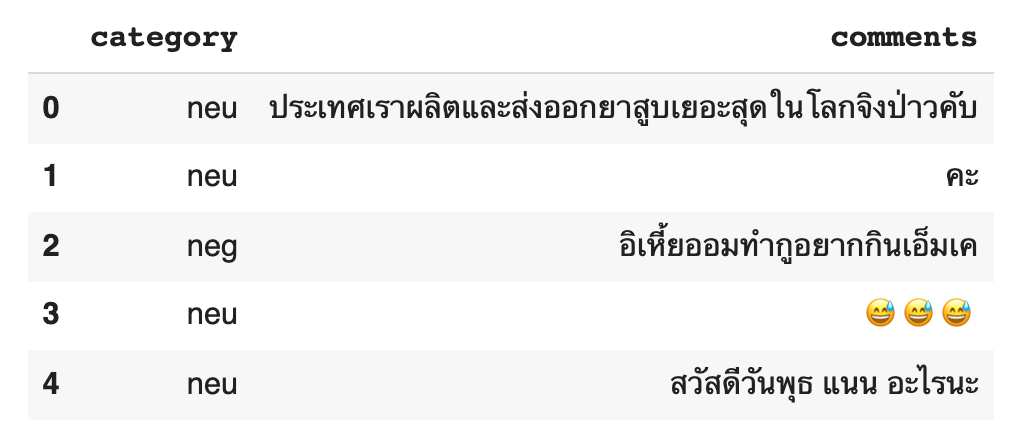

Data Preparation

ลบแถวที่ซ้ำ

df = df.drop_duplicates()

Sample ข้อมูล neu, pos และ neg อย่างละ 4300 แถว

neu_df = df[df.category == "neu"].sample(4300)
neu_df.head()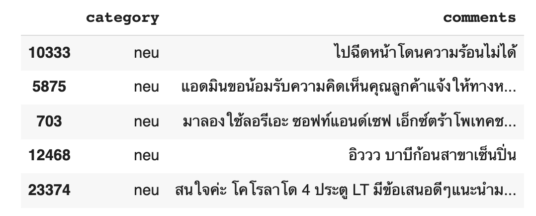

pos_df = df[df.category == "pos"]
pos_df.head()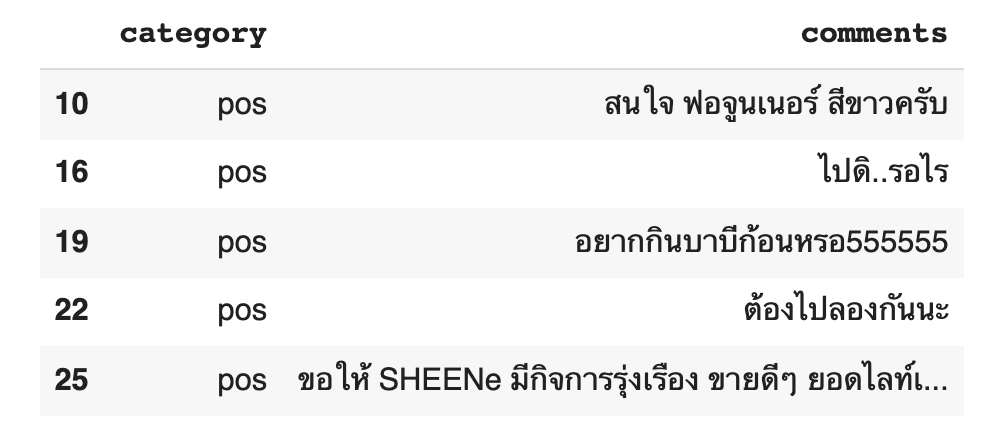

neg_df = df[df.category == "neg"].sample(4300)
neg_df.head()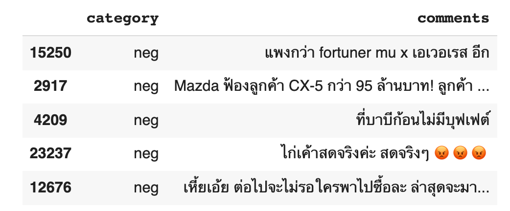

รวม neg และ pos

sentiment_df = pd.concat([neg_df, pos_df])
sentiment_df.head()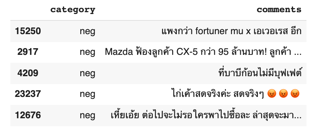

ปรับตัวอักษรภาษาอังกฤษ ให้เป็นอักษรตัวเล็ก ทั้งหมด

sentiment_df['clean_comments'] = sentiment_df['comments'].fillna('').apply(lambda x: x.lower())
sentiment_df.head()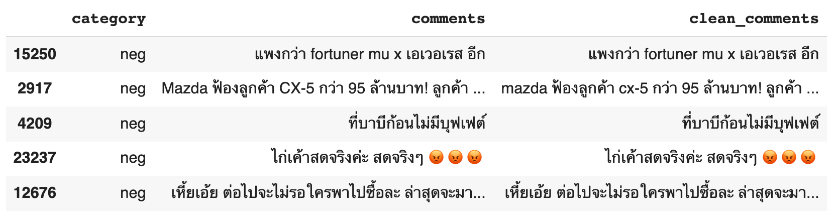

กำหนดอักขระที่ไม่ต้องการ

pun = '"#\'()*,-.;<=>[\\]^_`{|}~'
pun

"#'()*,-.;<=>[\]^_`{|}~

ลบอักขระที่ไม่ต้องการ

sentiment_df['clean_comments'] = sentiment_df['clean_comments'].str.replace(r'[%s]' % (pun), '', regex=True)

sentiment_df.sample(5)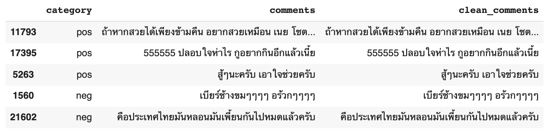

custom_words_list = set(thai_words())
len(custom_words_list)

62143

text = "โอเคบ่พวกเรารักภาษาบ้านเกิด"custom_tokenizer = Tokenizer(custom_words_list)custom_tokenizer.word_tokenize(text)

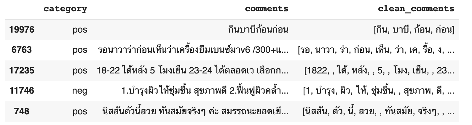
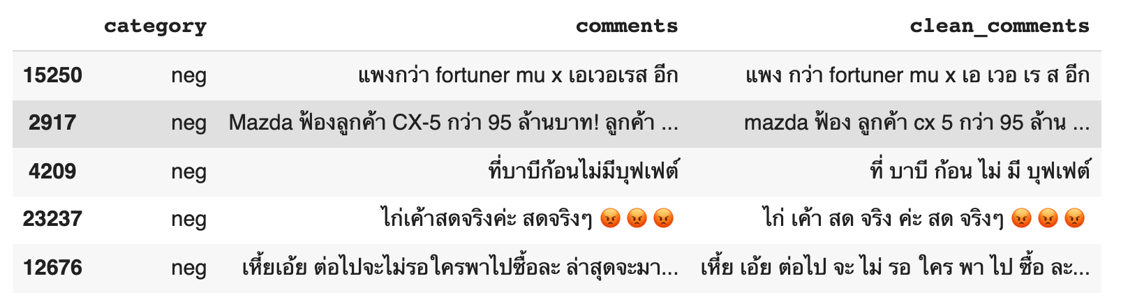
sentiment_df['clean_comments'] = sentiment_df['clean_comments'].apply(lambda x: custom_tokenizer.word_tokenize(x))

sentiment_df.sample(5)

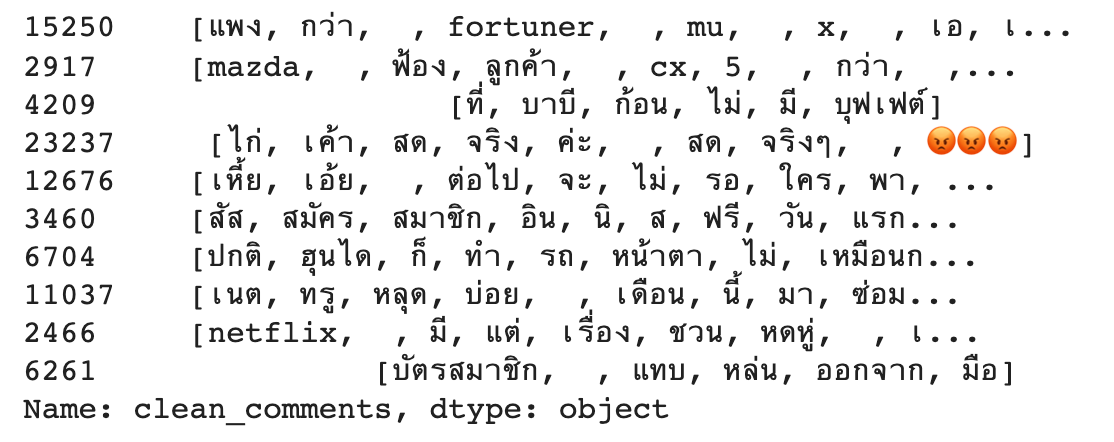
tokenized_doc = sentiment_df['clean_comments']
tokenized_doc[:10]

tokenized_doc = tokenized_doc.apply(lambda x: [item for item in x if item not in stop_words])

tokenized_doc[:10]

tokenized_doc = tokenized_doc.to_list()

# de-tokenization
detokenized_doc = []
for i in range(len(tokenized_doc)):
#     print(tokenized_doc[i])
    t = ' '.join(tokenized_doc[i])
    detokenized_doc.append(t)
    
sentiment_df['clean_comments'] = detokenized_doc

sentiment_df.head()

cleaned_words = sentiment_df['clean_comments'].to_list()

cleaned_words[:1]

def create_tokenizer(words, filters = ''):
    token = KRTokenizer()
    token.fit_on_texts(words)
    return token

train_word_tokenizer = create_tokenizer(cleaned_words)
vocab_size = len(train_word_tokenizer.word_index) + 1

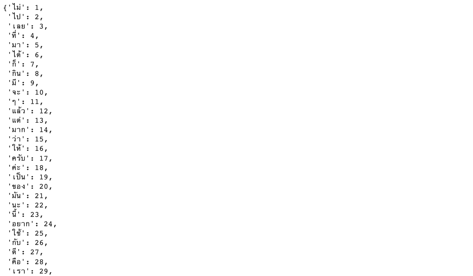
train_word_tokenizer.word_index

def max_length(words):
    return(len(max(words, key = len)))

max_length = max_length(tokenized_doc)
max_length

507

def encoding_doc(token, words):
    return(token.texts_to_sequences(words))

encoded_doc = encoding_doc(train_word_tokenizer, cleaned_words)

print(cleaned_words[0])
print(encoded_doc[0])

def padding_doc(encoded_doc, max_length):
   return(pad_sequences(encoded_doc, maxlen = max_length, padding = "post"))

padded_doc = padding_doc(encoded_doc, max_length)
print("Shape of padded docs = ",padded_doc.shape)

print(cleaned_words[0])
print(encoded_doc[0])
print(padded_doc[0])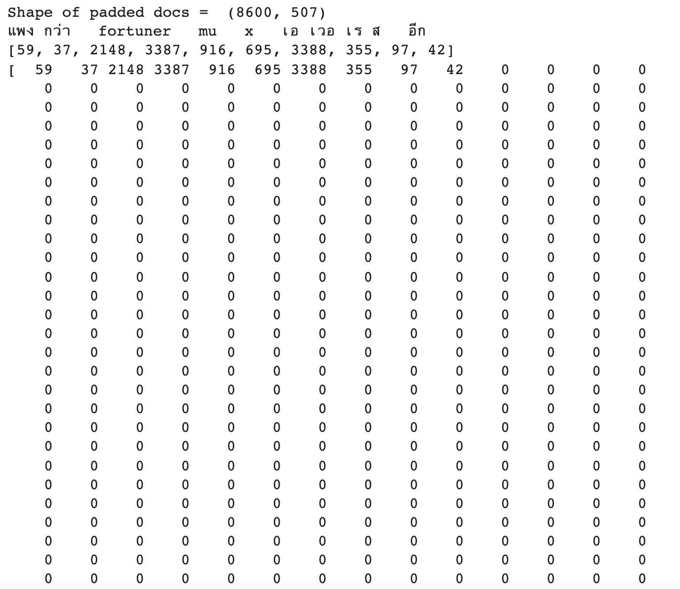

category = sentiment_df['category'].to_list()

unique_category = list(set(category))
unique_category

['pos', 'neg']

output_tokenizer = create_tokenizer(unique_category)

encoded_output = encoding_doc(output_tokenizer, category)
print(category[0:2])
print(encoded_output[0:2])

encoded_output = np.array(encoded_output).reshape(len(encoded_output), 1)
encoded_output.shape

(8600, 1)

def one_hot(encode):
  oh = OneHotEncoder(sparse = False)
  return(oh.fit_transform(encode))

output_one_hot = one_hot(encoded_output)
print(encoded_output[0])
print(output_one_hot[0])

แบ่งข้อมูล Train และ Validate

train_X, val_X, train_Y, val_Y = train_test_split(padded_doc, output_one_hot, shuffle = True, test_size = 0.2, stratify=output_one_hot)

print("Shape of train_X = %s and train_Y = %s" % (train_X.shape, train_Y.shape))
print("Shape of val_X = %s and val_Y = %s" % (val_X.shape, val_Y.shape))

Shape of train_X = (6880, 507) and train_Y = (6880, 2)

Shape of val_X = (1720, 507) and val_Y = (1720, 2)

num_classes = len(unique_category)

CNN Model for Sentiment Analysis using Word Embedding with Keras

#from tensorflow.keras.optimizers import Adam
#adam = Adam(learning_rate=0.0001)

from tensorflow.keras.optimizers.legacy import Adam
adam = Adam(learning_rate=0.0001)

นิยาม Model

# define the model
def define_model(length, vocab_size):
    # channel 1
    inputs1 = tf.keras.layers.Input(shape=(length,))
    embedding1 = tf.keras.layers.Embedding(vocab_size, DIMENSION, trainable = True)(inputs1)
    conv1 = tf.keras.layers.Conv1D(filters=32, kernel_size=4, activation='relu')(embedding1)
    drop1 = tf.keras.layers.Dropout(0.5)(conv1)
    pool1 = tf.keras.layers.MaxPooling1D(pool_size=2)(drop1)
    flat1 = tf.keras.layers.Flatten()(pool1)
    # channel 2
    inputs2 = tf.keras.layers.Input(shape=(length,))
    embedding2 = tf.keras.layers.Embedding(vocab_size, DIMENSION, trainable = True)(inputs2)
    conv2 = tf.keras.layers.Conv1D(filters=32, kernel_size=6, activation='relu')(embedding2)
    drop2 = tf.keras.layers.Dropout(0.5)(conv2)
    pool2 = tf.keras.layers.MaxPooling1D(pool_size=2)(drop2)
    flat2 = tf.keras.layers.Flatten()(pool2)
    # channel 3
    inputs3 = tf.keras.layers.Input(shape=(length,))
    embedding3 = tf.keras.layers.Embedding(vocab_size, DIMENSION, trainable = True)(inputs3)
    conv3 = tf.keras.layers.Conv1D(filters=32, kernel_size=8, activation='relu')(embedding3)
    drop3 = tf.keras.layers.Dropout(0.5)(conv3)
    pool3 = tf.keras.layers.MaxPooling1D(pool_size=2)(drop3)
    flat3 = tf.keras.layers.Flatten()(pool3)
    # merge
    merged = tf.keras.layers.concatenate([flat1, flat2, flat3])
    # interpretation
    dense1 = tf.keras.layers.Dense(10, activation='relu')(merged)
    outputs = tf.keras.layers.Dense(num_classes, activation='softmax')(dense1)
    model = Model(inputs=[inputs1, inputs2, inputs3], outputs=outputs)
    # compile
    model.compile(loss='categorical_crossentropy', optimizer=adam, metrics=['accuracy'])
    # summarize
    print(model.summary())
#     plot_model(model, show_shapes=True, to_file='multichannel.png')
    return model

model = define_model(max_length, vocab_size)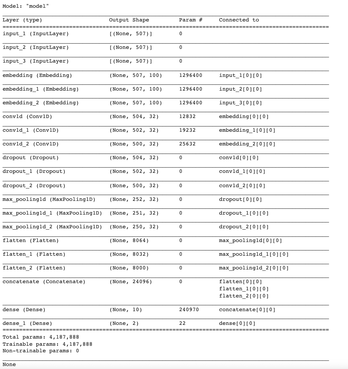

กำหนดจุด Check Point

filename = 'model.h5'
checkpoint = ModelCheckpoint(filename, monitor='val_loss', verbose=1, save_best_only=True, mode='min')

ใช้ ReduceLROnPlateau เพื่อปรับ Learning Rate

learning_rate_reduction = ReduceLROnPlateau(monitor='val_loss', patience = 3, verbose=1,factor=0.1, min_lr=0.000001)
callbacks_list = [checkpoint, learning_rate_reduction]

hist = model.fit([train_X, train_X, train_X], train_Y, epochs = EPOCHS, batch_size = BS, validation_data = ([val_X, val_X, val_X], val_Y), callbacks = [callbacks_list], shuffle=True)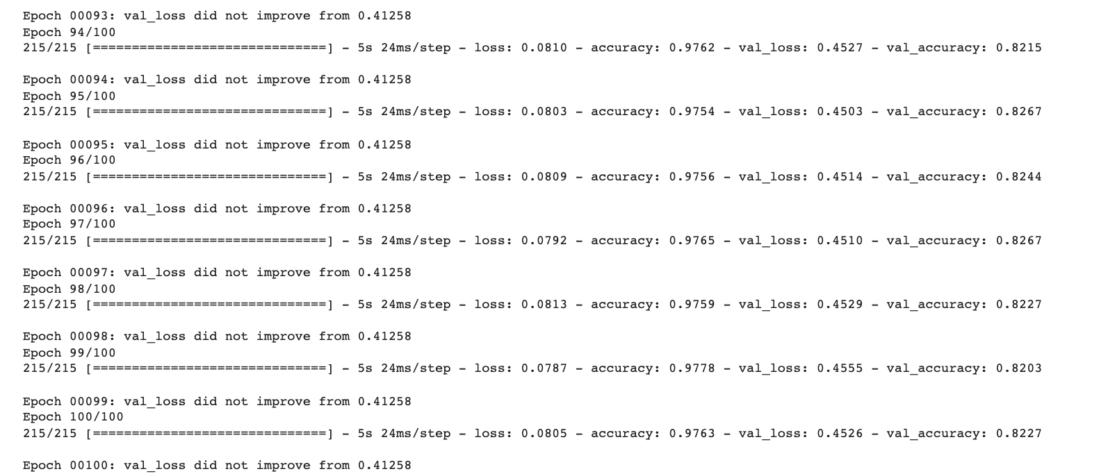

h1 = go.Scatter(y=hist.history['loss'], 
                    mode="lines", line=dict(
                    width=2,
                    color='blue'),
                    name="loss"
                   )
h2 = go.Scatter(y=hist.history['val_loss'], 
                    mode="lines", line=dict(
                    width=2,
                    color='red'),
                    name="val_loss"
                   )

data = [h1,h2]
layout1 = go.Layout(title='Loss',
                   xaxis=dict(title='epochs'),
                   yaxis=dict(title=''))
fig1 = go.Figure(data = data, layout=layout1)
fig1.show()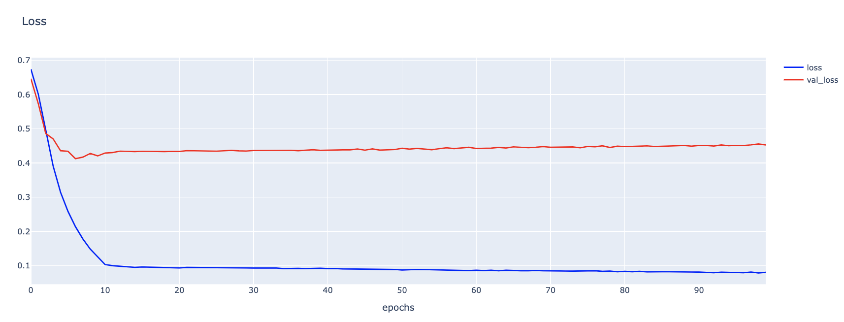

h1 = go.Scatter(y=hist.history['accuracy'], 
                    mode="lines", line=dict(
                    width=2,
                    color='blue'),
                    name="acc"
                   )
h2 = go.Scatter(y=hist.history['val_accuracy'], 
                    mode="lines", line=dict(
                    width=2,
                    color='red'),
                    name="val_acc"
                   )

data = [h1,h2]
layout1 = go.Layout(title='Accuracy',
                   xaxis=dict(title='epochs'),
                   yaxis=dict(title=''))
fig1 = go.Figure(data = data, layout=layout1)
fig1.show()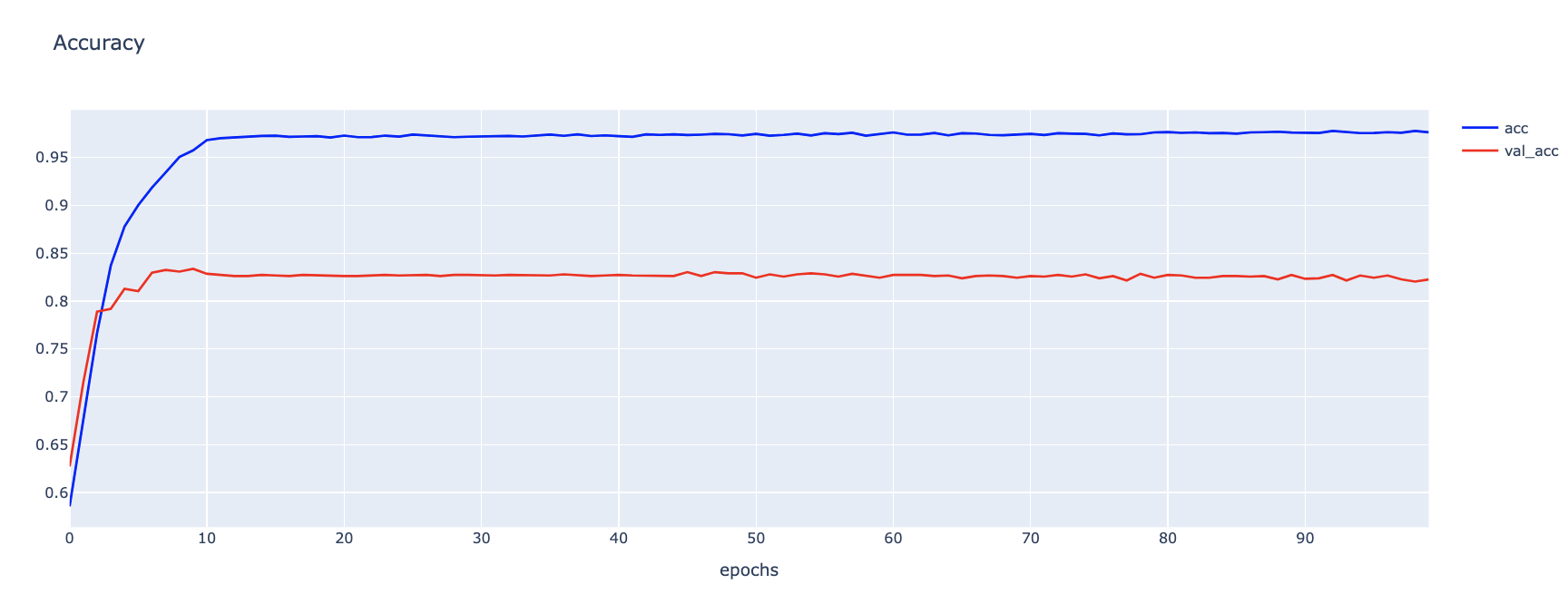

predict_model = load_model(filename) 
predict_model.summary()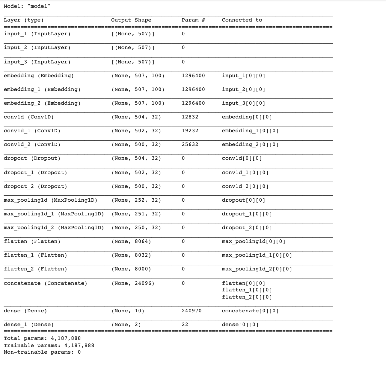

score = predict_model.evaluate([val_X, val_X, val_X], val_Y, verbose=0)
print('Validate loss:', score[0])
print('Validate accuracy:', score[1])

Validate loss: 0.41258129477500916

Validate accuracy: 0.8296511769294739

predicted_classes = np.argmax(predict_model.predict([val_X, val_X, val_X]), axis=-1)
predicted_classes.shape

(1720,)

y_true = np.argmax(val_Y,axis = 1)
print(val_Y[0])
print(y_true[0])

cm = confusion_matrix(y_true, predicted_classes)
np.savetxt("confusion_matrix.csv", cm, delimiter=",")

df_cm = pd.DataFrame(cm, range(2), range(2))
plt.figure(figsize=(20,14))
sn.set(font_scale=1.2) # for label size
sn.heatmap(df_cm, annot=True, annot_kws={"size": 14}, fmt='g') # for num predict size

plt.show()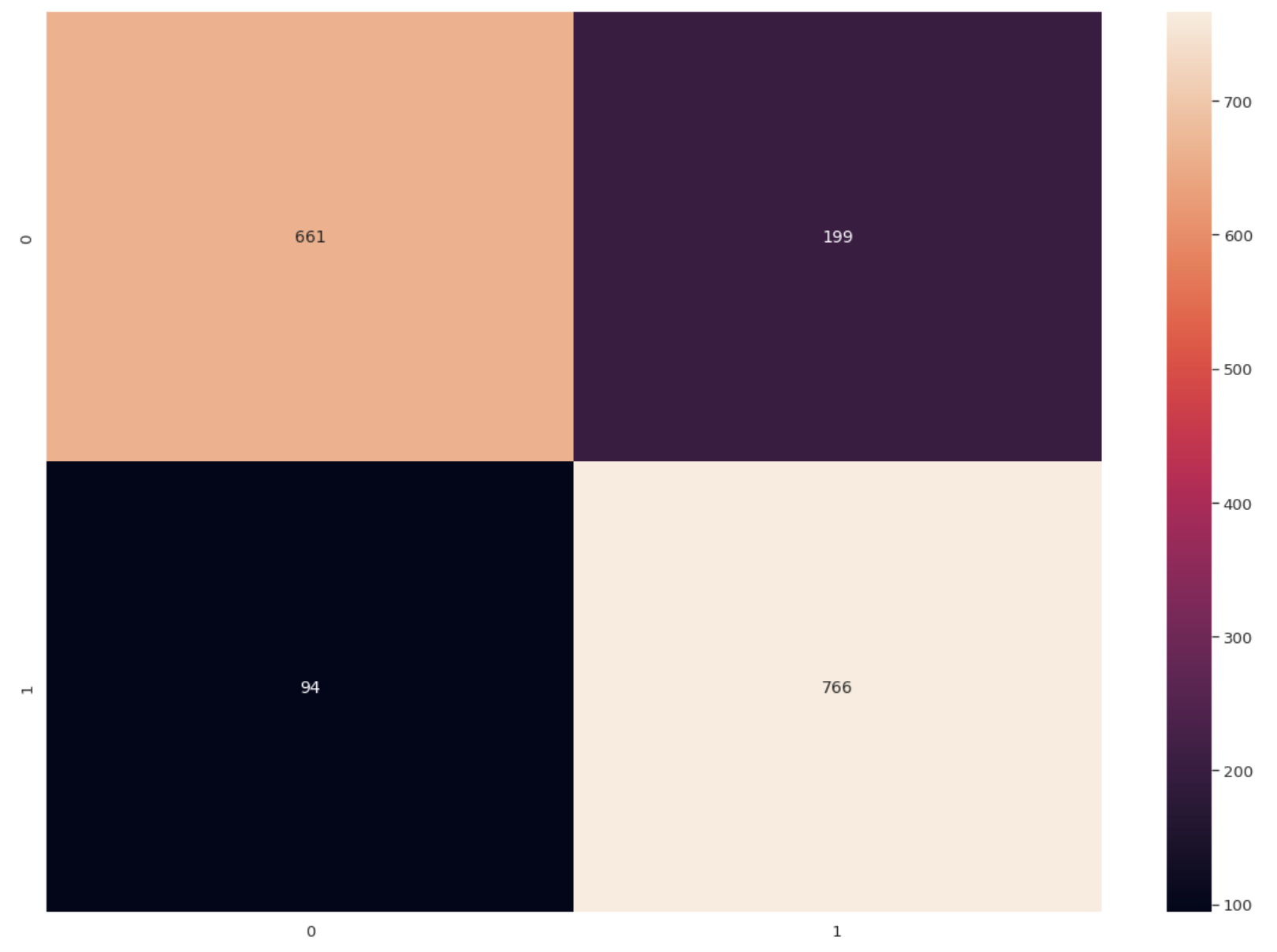

label_dict = output_tokenizer.word_index

label = [key for key, value in label_dict.items()]

print(classification_report(y_true, predicted_classes, target_names=label, digits=4))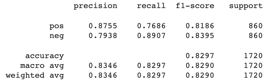

CNN Model for Sentiment Analysis using Word Embedding from Gensim

sentences = [st.split() for st in cleaned_words]

Train Word2Vec ด้วย Gensim

w2v_model = Word2Vec(sentences, min_count=1, vector_size=DIMENSION, workers=6, sg=1, epochs=500)

Save Word2Vec

w2v_model.save('w2v_model.bin')

เรียกใช้ Word2Vec

new_model = Word2Vec.load('w2v_model.bin')

เตรียม Embedding Matrix

embedding_matrix = np.zeros((vocab_size, DIMENSION))

for word, i in train_word_tokenizer.word_index.items():
    if word in new_model.wv.index_to_key:
        embedding_vector = new_model.wv[word]
        embedding_matrix[i] = embedding_vector

นิยาม Model

# define the model
def define_w2v_model(length, vocab_size, embedding_matrix):
    # channel 1
    inputs1 = tf.keras.layers.Input(shape=(length,))
    embedding1 = tf.keras.layers.Embedding(vocab_size, DIMENSION, trainable = False, weights=[embedding_matrix])(inputs1)
    conv1 = tf.keras.layers.Conv1D(filters=32, kernel_size=4, activation='relu')(embedding1)
    drop1 = tf.keras.layers.Dropout(0.5)(conv1)
    pool1 = tf.keras.layers.MaxPooling1D(pool_size=2)(drop1)
    flat1 = tf.keras.layers.Flatten()(pool1)
    # channel 2
    inputs2 = tf.keras.layers.Input(shape=(length,))
    embedding2 = tf.keras.layers.Embedding(vocab_size, DIMENSION, trainable = False, weights=[embedding_matrix])(inputs2)
    conv2 = tf.keras.layers.Conv1D(filters=32, kernel_size=6, activation='relu')(embedding2)
    drop2 = tf.keras.layers.Dropout(0.5)(conv2)
    pool2 = tf.keras.layers.MaxPooling1D(pool_size=2)(drop2)
    flat2 = tf.keras.layers.Flatten()(pool2)
    # channel 3
    inputs3 = tf.keras.layers.Input(shape=(length,))
    embedding3 = tf.keras.layers.Embedding(vocab_size, DIMENSION, trainable = False, weights=[embedding_matrix])(inputs3)
    conv3 = tf.keras.layers.Conv1D(filters=32, kernel_size=8, activation='relu')(embedding3)
    drop3 = tf.keras.layers.Dropout(0.5)(conv3)
    pool3 = tf.keras.layers.MaxPooling1D(pool_size=2)(drop3)
    flat3 = tf.keras.layers.Flatten()(pool3)
    # merge
    merged = tf.keras.layers.concatenate([flat1, flat2, flat3])
    # interpretation
    dense1 = tf.keras.layers.Dense(10, activation='relu')(merged)
    outputs = tf.keras.layers.Dense(num_classes, activation='softmax')(dense1)
    model = Model(inputs=[inputs1, inputs2, inputs3], outputs=outputs)
    # compile
    model.compile(loss='categorical_crossentropy', optimizer=adam, metrics=['accuracy'])
    # summarize
    print(model.summary())
#     plot_model(model, show_shapes=True, to_file='multichannel.png')
    return model

model2 = define_w2v_model(max_length, vocab_size, embedding_matrix)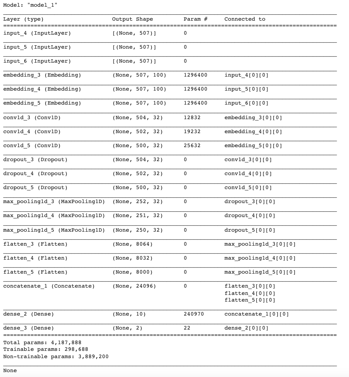

กำหนดจุด Check Point

filename = 'model2.h5'
checkpoint = ModelCheckpoint(filename, monitor='val_loss', verbose=1, save_best_only=True, mode='min')

ใช้ ReduceLROnPlateau เพื่อปรับ Learning Rate

learning_rate_reduction = ReduceLROnPlateau(monitor='val_loss', patience = 3, verbose=1,factor=0.1, min_lr=0.000001)
callbacks_list = [checkpoint, learning_rate_reduction]

hist2 = model2.fit([train_X, train_X, train_X], train_Y, epochs = EPOCHS, batch_size = BS, validation_data = ([val_X, val_X, val_X], val_Y), callbacks = [callbacks_list], shuffle=True)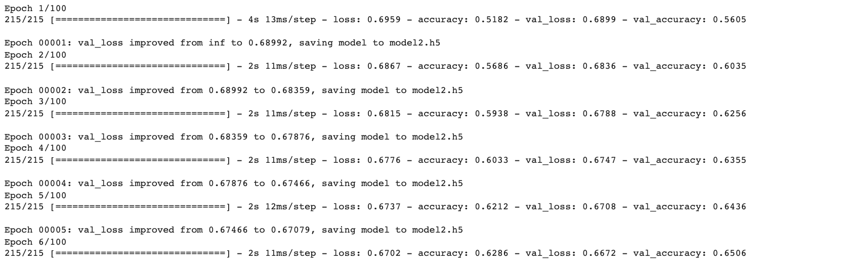

h1 = go.Scatter(y=hist2.history['loss'], 
                    mode="lines", line=dict(
                    width=2,
                    color='blue'),
                    name="loss"
                   )
h2 = go.Scatter(y=hist2.history['val_loss'], 
                    mode="lines", line=dict(
                    width=2,
                    color='red'),
                    name="val_loss"
                   )

data = [h1,h2]
layout1 = go.Layout(title='Loss',
                   xaxis=dict(title='epochs'),
                   yaxis=dict(title=''))
fig1 = go.Figure(data = data, layout=layout1)
fig1.show()

h1 = go.Scatter(y=hist2.history['loss'], 
                    mode="lines", line=dict(
                    width=2,
                    color='blue'),
                    name="loss"
                   )
h2 = go.Scatter(y=hist2.history['val_loss'], 
                    mode="lines", line=dict(
                    width=2,
                    color='red'),
                    name="val_loss"
                   )

data = [h1,h2]
layout1 = go.Layout(title='Loss',
                   xaxis=dict(title='epochs'),
                   yaxis=dict(title=''))
fig1 = go.Figure(data = data, layout=layout1)
fig1.show()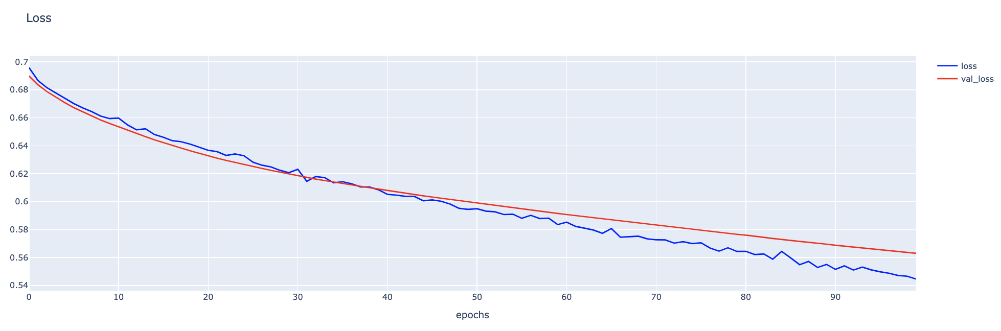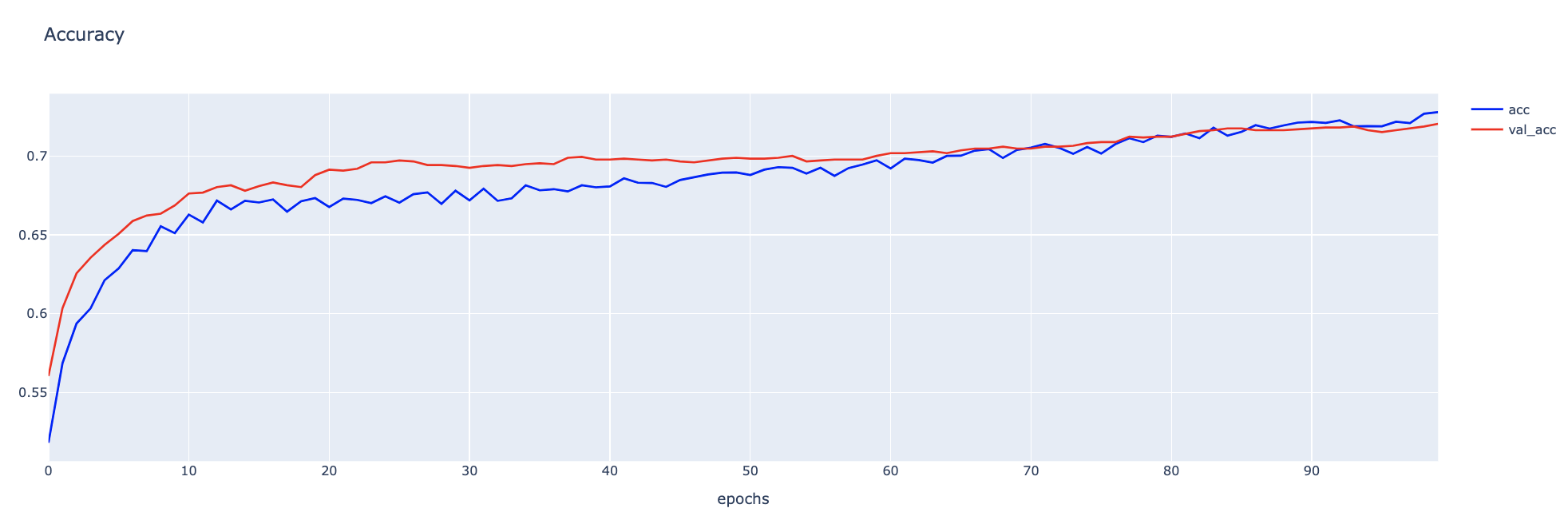

predict_model2 = load_model(filename) 
predict_model2.summary()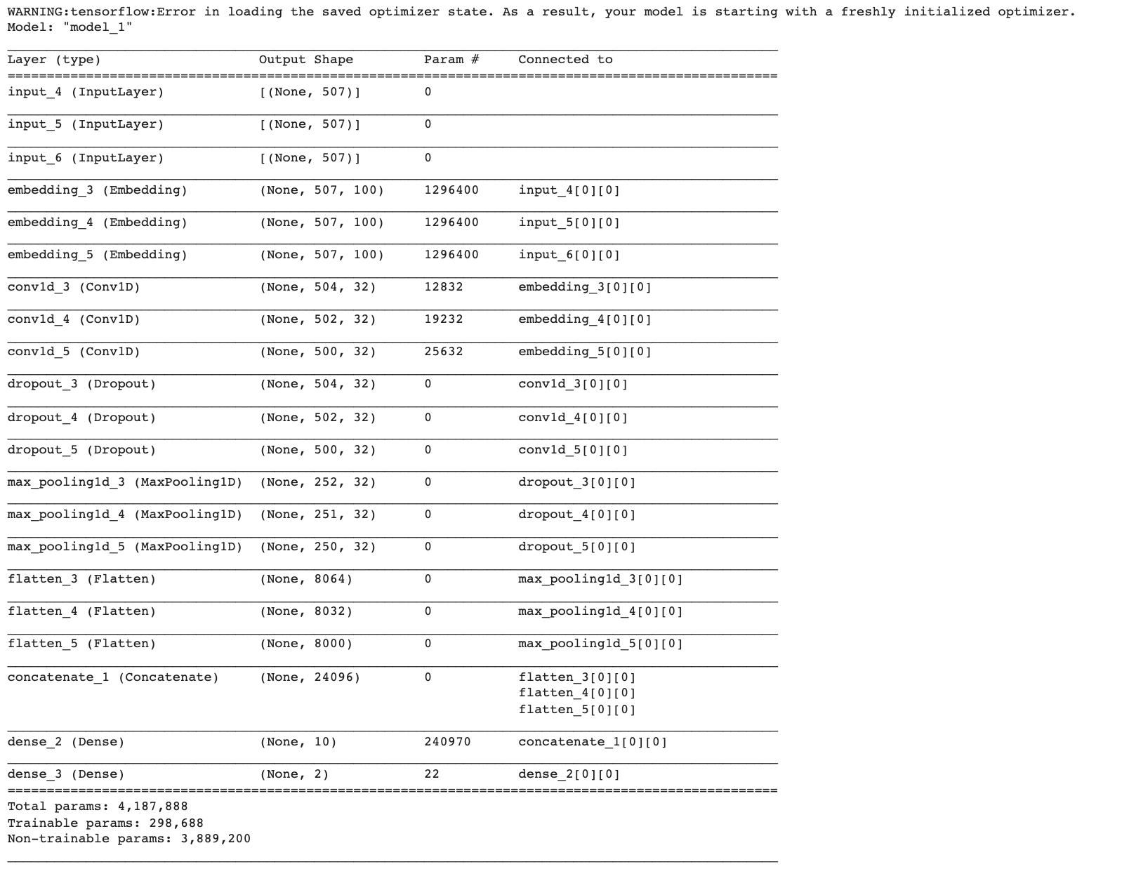

score = predict_model2.evaluate([val_X, val_X, val_X], val_Y, verbose=0)
print('Validate loss:', score[0])
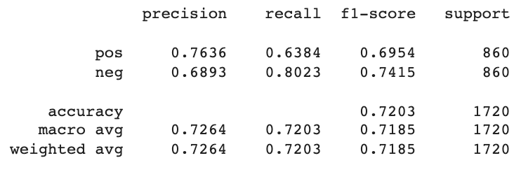
print('Validate accuracy:', score[1])

Validate loss: 0.5630149841308594

Validate accuracy: 0.7203488349914551

predicted_classes = np.argmax(predict_model2.predict([val_X, val_X, val_X]), axis=-1)
predicted_classes.shape

(1720,)

cm = confusion_matrix(y_true, predicted_classes)
np.savetxt("confusion_matrix.csv", cm, delimiter=",")

df_cm = pd.DataFrame(cm, range(2), range(2))
plt.figure(figsize=(20,14))
sn.set(font_scale=1.2) # for label size
sn.heatmap(df_cm, annot=True, annot_kws={"size": 14}, fmt='g') # for num predict size

plt.show()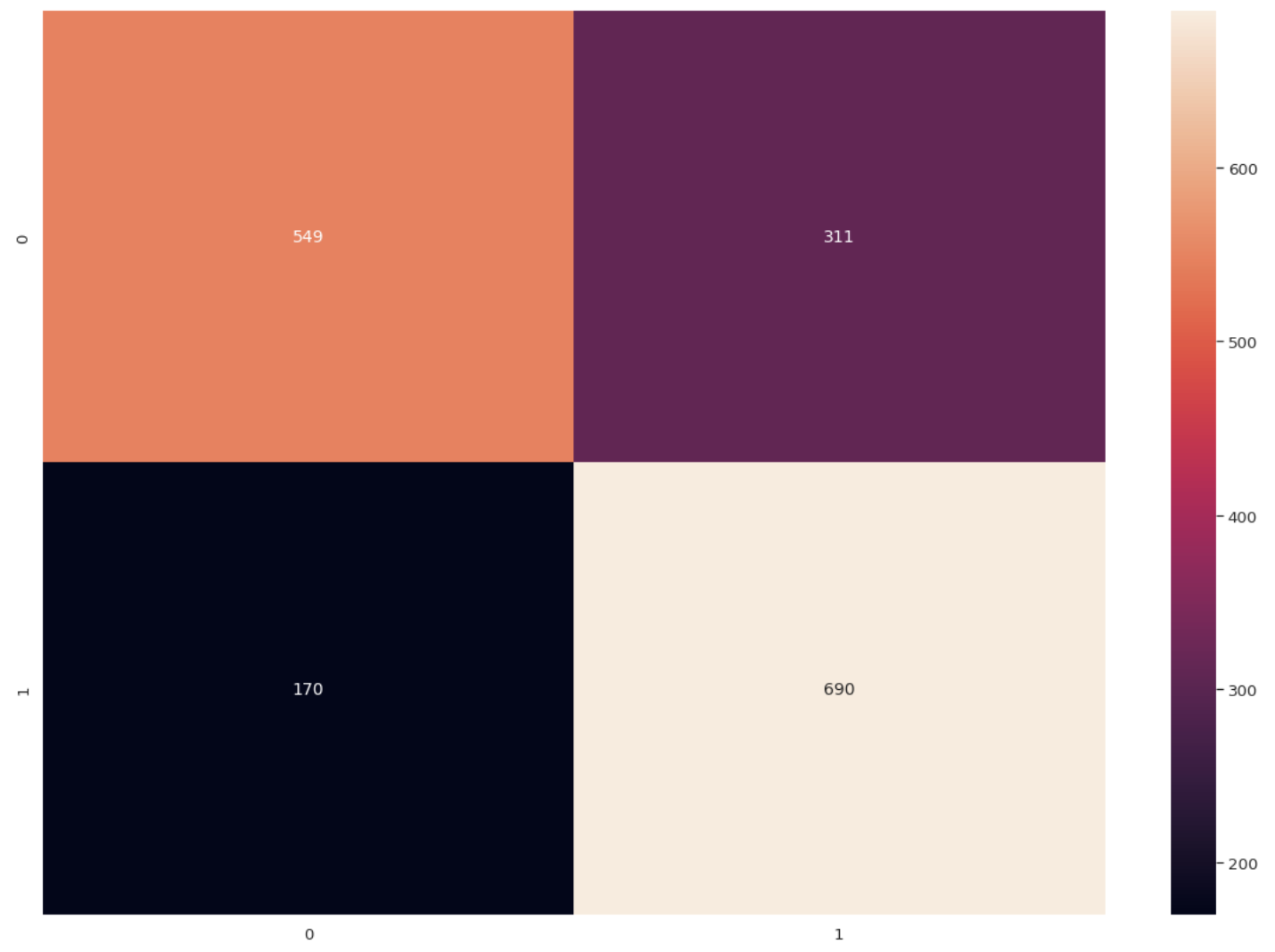

print(classification_report(y_true, predicted_classes, target_names=label, digits=4))