Sentiment Analysis 101

บทความโดย ผศ.ดร.ณัฐโชติ พรหมฤทธิ์
ภาควิชาคอมพิวเตอร์
คณะวิทยาศาสตร์
มหาวิทยาลัยศิลปากร

ใน Workshop นี้เราจะได้เรียนรู้เกี่ยวกับการทำ Sentiment Analysis โดยใช้ Model แบบ RNN ที่รับ Dataset ผ่าน Input Node แบบ Time Series หรือข้อมูลที่มีลักษณะเป็นลำดับ เช่น X0, X1, X2,... Xt

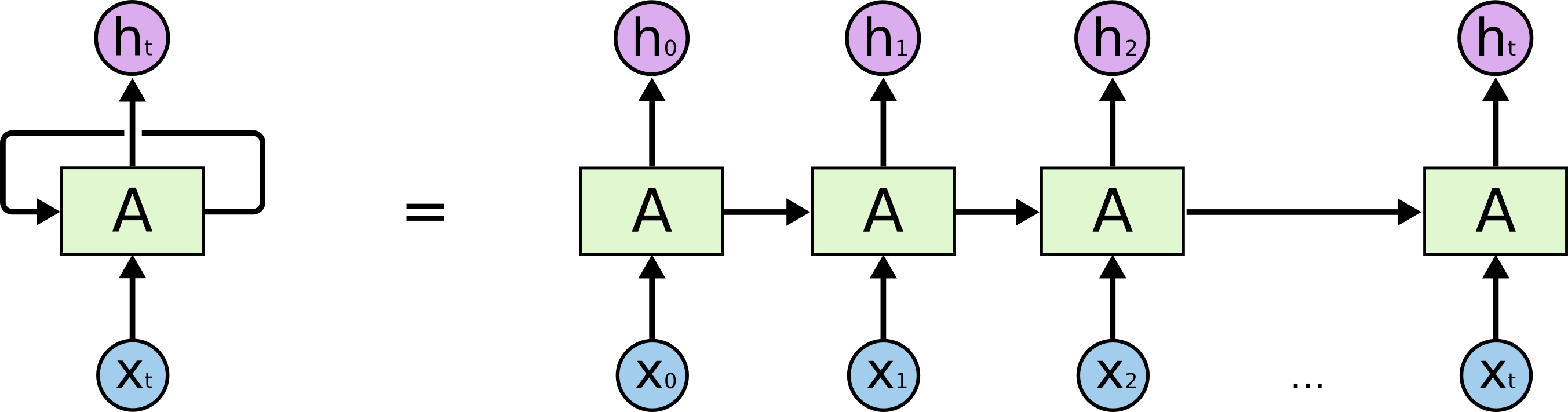
ซึ่งเมื่อมีการประมวลผลใน RNN Cell แล้ว จะมีการส่งผลลัพธ์ออกมาเป็น Vector h0, h1, h2,  ..., ht ตามลำดับ โดยในการประมวลผลแต่ละรอบจะมีการนำ Output State ของ RNN Cell ในรอบก่อนหน้ามาเป็น Input State ของ RNN Cell ในรอบถัดไป

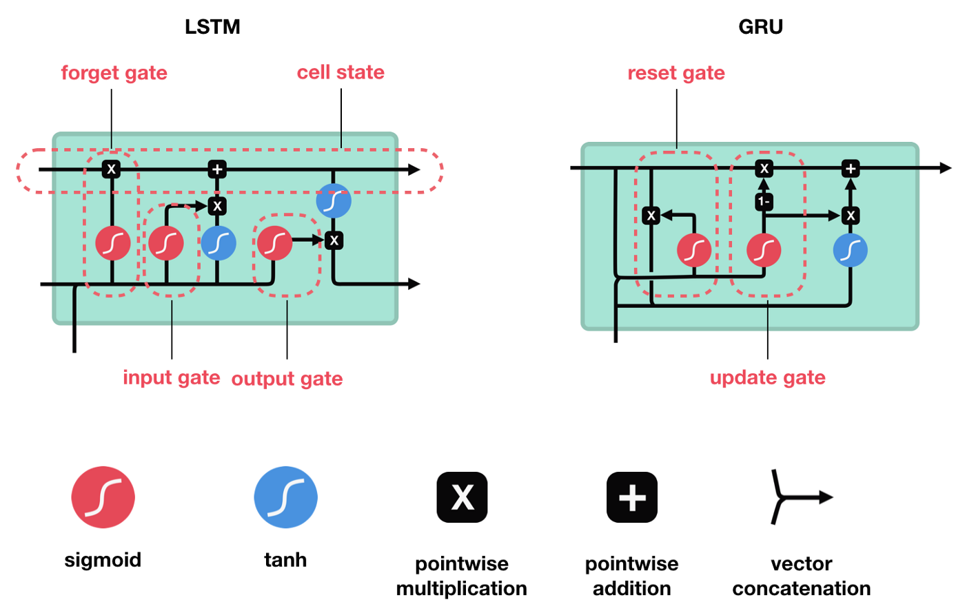
ภายใน RNN Cell จะมีวงจรสำหรับนำ Input Data x Weight ในรูปแบบต่างๆ ซึ่งปัจจุบันมีรูปแบบ RNN Cell ที่นิยม 2 รูปแบบ ได้แก่ วงจรแบบ LSTM และ GRU

อย่างไรก็ตาม RNN Neural Network นั้นมีจุดอ่อนที่มันจะมีการสูญเสีย Information เมื่อมีการย้อนกลับไปปรับค่า Weight โดยเฉพาะถ้ามีการรับ Input Data ที่มีความยาวมากๆ  ดังนั้นเพื่อลดการสูญเสีย Information ในการปรับค่า Weight เราจะประกอบ RNN Cell ในแบบ Bidirectional RNN ครับ

• Import Package ที่จำเป็น

import pandas as pd
import re
# from nltk.tokenize import word_tokenize
from pythainlp.tokenize import word_tokenize
from keras.preprocessing.text import Tokenizer

from keras.preprocessing.sequence import pad_sequences
from sklearn.preprocessing import OneHotEncoder
from sklearn.model_selection import train_test_split

import numpy as np

from tensorflow.keras.models import Sequential
from tensorflow.keras.layers import Dense, GRU, LSTM, Bidirectional, Embedding, Dropout, BatchNormalization
from tensorflow.keras.models import load_model
from tensorflow.keras.callbacks import ModelCheckpoint

from tensorflow.keras.optimizers import Adam

import seaborn as sn
import matplotlib.pyplot as plt

import pickle as p
import plotly
import plotly.graph_objs as go

from sklearn.metrics import confusion_matrix

from sklearn.metrics import classification_report

• กำหนดจำนวน EPOCHS และ Batch Size ดังต่อไปนี้

EPOCHS = 10
BS = 32

• Load Dataset ซึ่งประกอบด้วย ข้อความ (comments), ผลเฉลย (labels)

comments = []
labels = []

with open("train.txt",encoding="utf-8") as f:
    for line in f:
        comments.append(line.strip())

with open("train_label.txt",encoding="utf-8") as f:
    for line in f:
        labels.append(line.strip())

df = pd.DataFrame({ "category": labels, "comments": comments })
df.head()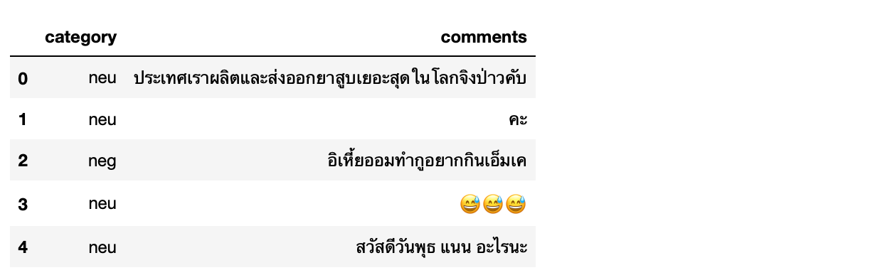

• ลบแถวที่ซ้ำ

df = df.drop_duplicates()

• Sample ข้อมูล neu, pos และ neg อย่างละ 4300 แถว

neu_df = df[df.category == "neu"].sample(4300)
neu_df.head()

pos_df = df[df.category == "pos"]
pos_df.head()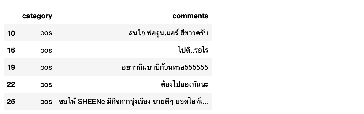

neg_df = df[df.category == "neg"].sample(4300)
neg_df.head()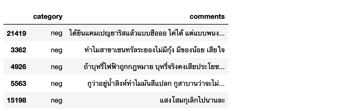

• รวม neg และ pos

sentiment_df = pd.concat([neg_df, pos_df])
sentiment_df.head()

comments = sentiment_df.comments.values
comments.shape

comments[0]

category = sentiment_df.category.values
category.shape

• นิยาม Function เพื่อ Cleaning ประโยค โดยคัดไว้เฉพาะข้อความภาษาไทยตัดคำ แปลงเป็นตัวอักษรตัวเล็ก เก็บแต่ละคำของแต่ละประโยคไว้ใน List (temp) เพื่อหาความยาวของประโยค รวมทั้งเก็บแต่ละประโยคแบบ String (words) เพื่อสร้าง Train Data

def cleaning(sentences):
  words = []
  temp = []
  for s in sentences:
    clean = re.sub(r'[^ก-๙]', "", s)
    w = word_tokenize(clean)
    temp.append([i.lower() for i in w])
    words.append(' '.join(w).lower())
    
  return words, temp

• Clean ประโยคทั้งหมด

cleaned_words, temp = cleaning(comments)
print(len(cleaned_words))
print(cleaned_words[:5])

• นิยาม Function create_tokenizer เพื่อสร้าง Keras TokenizerObject

def create_tokenizer(words, filters = ''):
    token = Tokenizer(filters=filters)
    token.fit_on_texts(words)
    return token

• สร้าง Keras Tokenizer Object ที่มีการ Train ด้วย Sentence ที่ถูก Cleaning แล้ว ซึ่งเราจะได้ Bag of Word และจำนวนคำศัพท์ของ Bag of Word จาก Keras Tokenizer ดังภาพด้านล่าง

train_word_tokenizer = create_tokenizer(cleaned_words)
vocab_size = len(train_word_tokenizer.word_index) + 1

train_word_tokenizer.word_index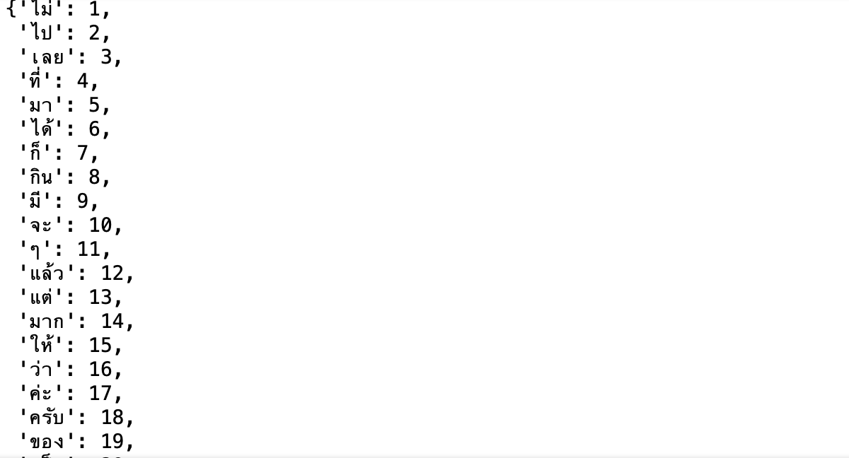

• นิยาม Function เพื่อหาความยาวสูงสุดของคำในประโยค ซึ่งเราจะค้นหาประโยคที่มีความยาวสูงสูดโดยใช้  Parameter key = len และนับคำในประโยคโดยใช้ Function len

def max_length(words):
    return(len(max(words, key = len)))

• กำหนดความยาวสูงสุดของคำในประโยคให้กับ max_length เพื่อเตรียมทำ Padding และกำหนดจำนวน Step ของ GRU Network ซึ่งพบว่าประโยคยาวที่สุดมีความยาว 361 คำ

max_length = max_length(temp)
max_length

• นิยาม Function เพื่อแปลงคำเป็นตัวเลข

def encoding_doc(token, words):
    return(token.texts_to_sequences(words))

• แปลงคำในประโยคที่ได้ทำ Cleaning เป็นตัวเลข ด้วย Keras Tokenizer Object ที่ถูก Train แล้ว

encoded_doc = encoding_doc(train_word_tokenizer, cleaned_words)

print(cleaned_words[0])
print(encoded_doc[0])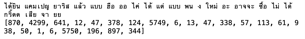

• นิยาม Function เพื่อทำ Padding ตัวเลขที่แทนแต่ละคำในประโยค โดยกำหนดให้มีการเติม 0 เพื่อให้แต่ละประโยคมีความยาวเท่ากัน (361 คำ)

def padding_doc(encoded_doc, max_length):
    return(pad_sequences(encoded_doc, maxlen = max_length, padding = "post"))

• ทำ Padding

padded_doc = padding_doc(encoded_doc, max_length)
print("Shape of padded docs = ",padded_doc.shape)

print(cleaned_words[0])
print(encoded_doc[0])
print(padded_doc[0])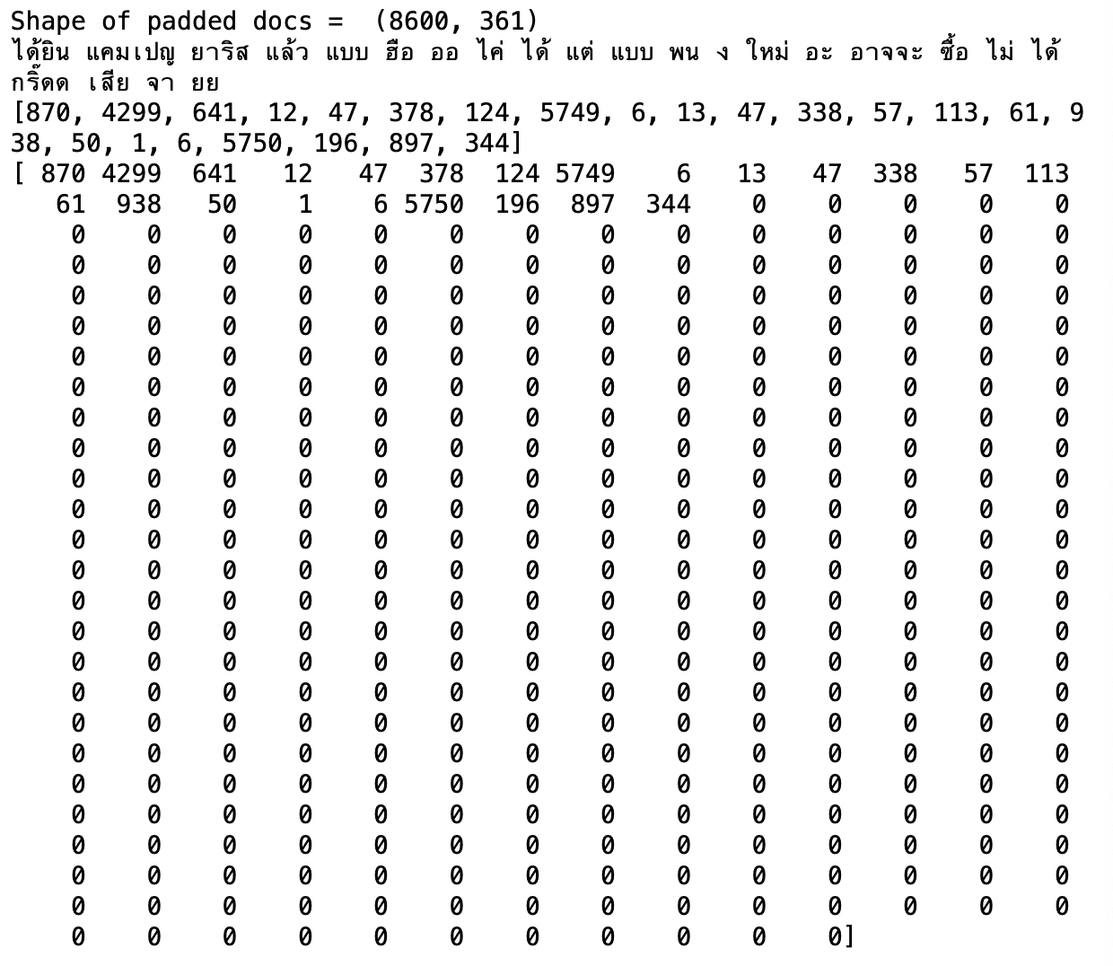

unique_category = list(set(category))
unique_category

• สร้าง output_tokenizer ด้วยการ Train tokenizer ด้วยชื่อ Class ทั้งหมด 2 Class

output_tokenizer = create_tokenizer(unique_category)

• แปลงผลเฉลยเป็นตัวเลขโดยใช้ output_tokenizer

encoded_output = encoding_doc(output_tokenizer, category)
print(category[0:2])
print(encoded_output[0:2])

• เพิ่มมิติของผลเฉลยจาก 8600 เป็น 8600 x 1 สำหรับการเข้ารหัสผลเฉลยแบบ One Hot

encoded_output = np.array(encoded_output).reshape(len(encoded_output), 1)
encoded_output.shape

• นิยาม Function การเข้ารหัสผลเฉลยแบบ One Hot

def one_hot(encode):
  oh = OneHotEncoder(sparse = False)
  return(oh.fit_transform(encode))

• เข้ารหัสผลเฉลยแบบ One Hot

output_one_hot = one_hot(encoded_output)
print(encoded_output[0])
print(output_one_hot[0])

• แบ่ง Input Data พร้อมผลเฉลย (Dataset) สำหรับ Train 80% และ Validate 20% โดยใช้ Parameter แบบ Stratified Sampling เพื่อให้มั่นใจว่าจะได้ Validate Dataset ที่มีข้อมูลครบทุก Intent

train_X, val_X, train_Y, val_Y = train_test_split(padded_doc, output_one_hot, shuffle = True, test_size = 0.2, stratify=output_one_hot)

• Print Shape ของ Dataset

print("Shape of train_X = %s and train_Y = %s" % (train_X.shape, train_Y.shape))
print("Shape of val_X = %s and val_Y = %s" % (val_X.shape, val_Y.shape))

• กำหนดจำนวน Intent ให้กับ num_classes สำหรับนิยามจำนวน Output Node ของ GRU Neural Network

num_classes = len(unique_category)

นิยาม Model แบบ GRU

• นิยาม Model แบบ GRU ซึ่งเป็น Recurrent Neural Network (RNN) แบบหนึ่ง โดยกำหนดค่า learning rate (lr) ให้เป็น 0.0001  (ใน colab ให้ใช้ learning_rate แทน lr)

from tensorflow.keras.models import Sequential
from tensorflow.keras.layers import Dense, GRU, LSTM, Bidirectional, Embedding, Dropout, BatchNormalization
from tensorflow.keras.models import load_model

from tensorflow.keras.optimizers import Adam
adam = Adam(lr=0.0001)

def create_model(vocab_size, max_length):
  model = Sequential()
  
  model.add(Embedding(vocab_size, 128, input_length = max_length,  trainable = True))
  model.add(Bidirectional(GRU(128, activation = "relu"))) # activation = "relu"
  model.add(Dense(128, activation = "relu"))
  model.add(Dropout(0.5))
  model.add(Dense(64, activation = "relu"))
  model.add(Dropout(0.5))
  model.add(BatchNormalization())
  model.add(Dense(num_classes, activation = "softmax"))
  
  return model
  
model = create_model(vocab_size, max_length)

• Compile และ Print ชนิดของ Layer, Output Shape และจำนวน Parameter ของ Model

model.compile(loss = "categorical_crossentropy", optimizer = adam, metrics = ["accuracy"])
model.summary()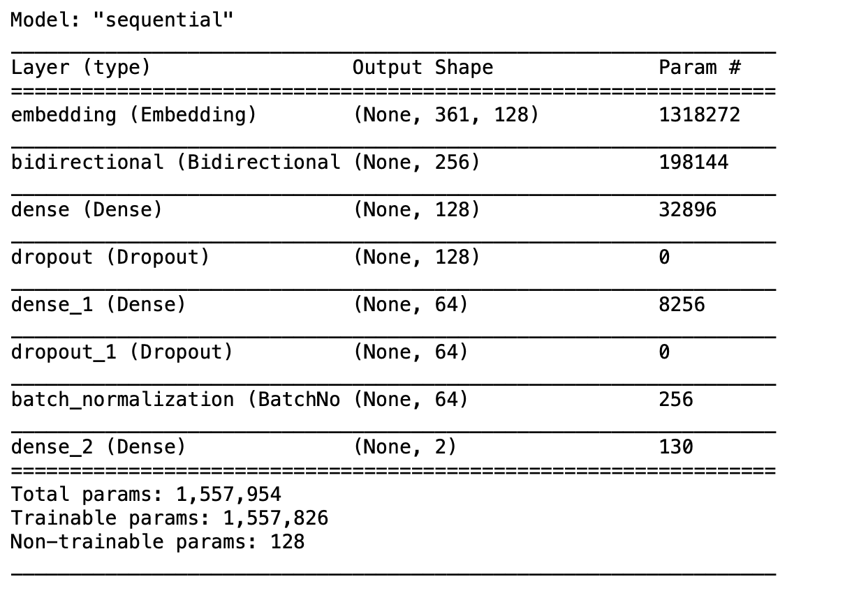

• สร้างจุด Check Point เพื่อ Save Model เฉพาะ Epoch ที่มี val_loss น้อยที่สุด

filename = 'model.h5'
checkpoint = ModelCheckpoint(filename, monitor='val_loss', verbose=1, save_best_only=True, mode='min')

• Train Model

hist = model.fit(train_X, train_Y, epochs = EPOCHS, batch_size = BS, validation_data = (val_X, val_Y), callbacks = [checkpoint])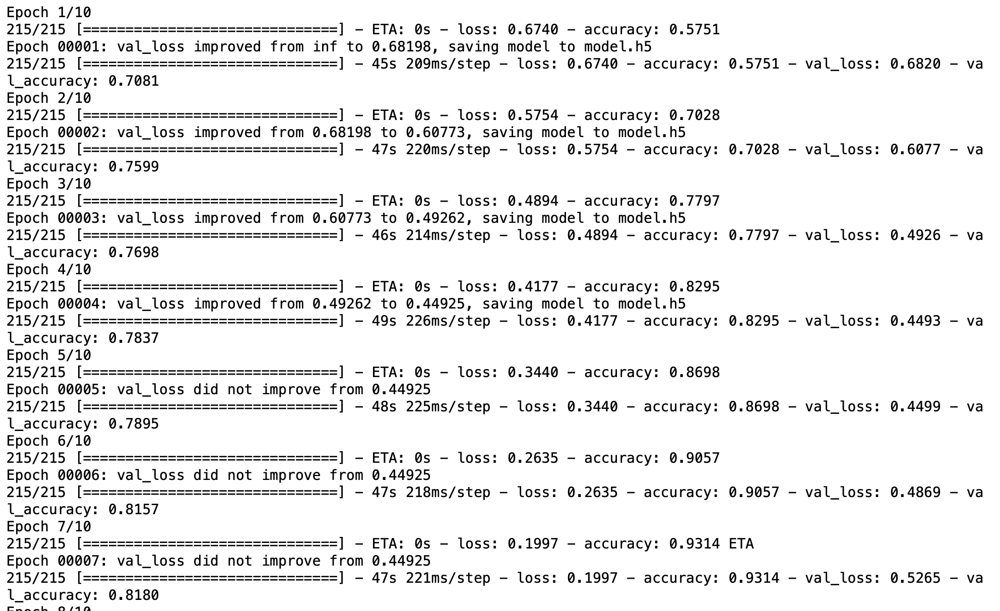

• Save History

with open('history_model', 'wb') as file:
    p.dump(hist.history, file)

• Load History

with open('history_model', 'rb') as file:
    his = p.load(file)

• Plot Loss และ Validate Loss

h1 = go.Scatter(y=his['loss'], 
                    mode="lines", line=dict(
                    width=2,
                    color='blue'),
                    name="loss"
                   )
h2 = go.Scatter(y=his['val_loss'], 
                    mode="lines", line=dict(
                    width=2,
                    color='red'),
                    name="val_loss"
                   )

data = [h1,h2]
layout1 = go.Layout(title='Loss',
                   xaxis=dict(title='epochs'),
                   yaxis=dict(title=''))
fig1 = go.Figure(data = data, layout=layout1)
fig1.show()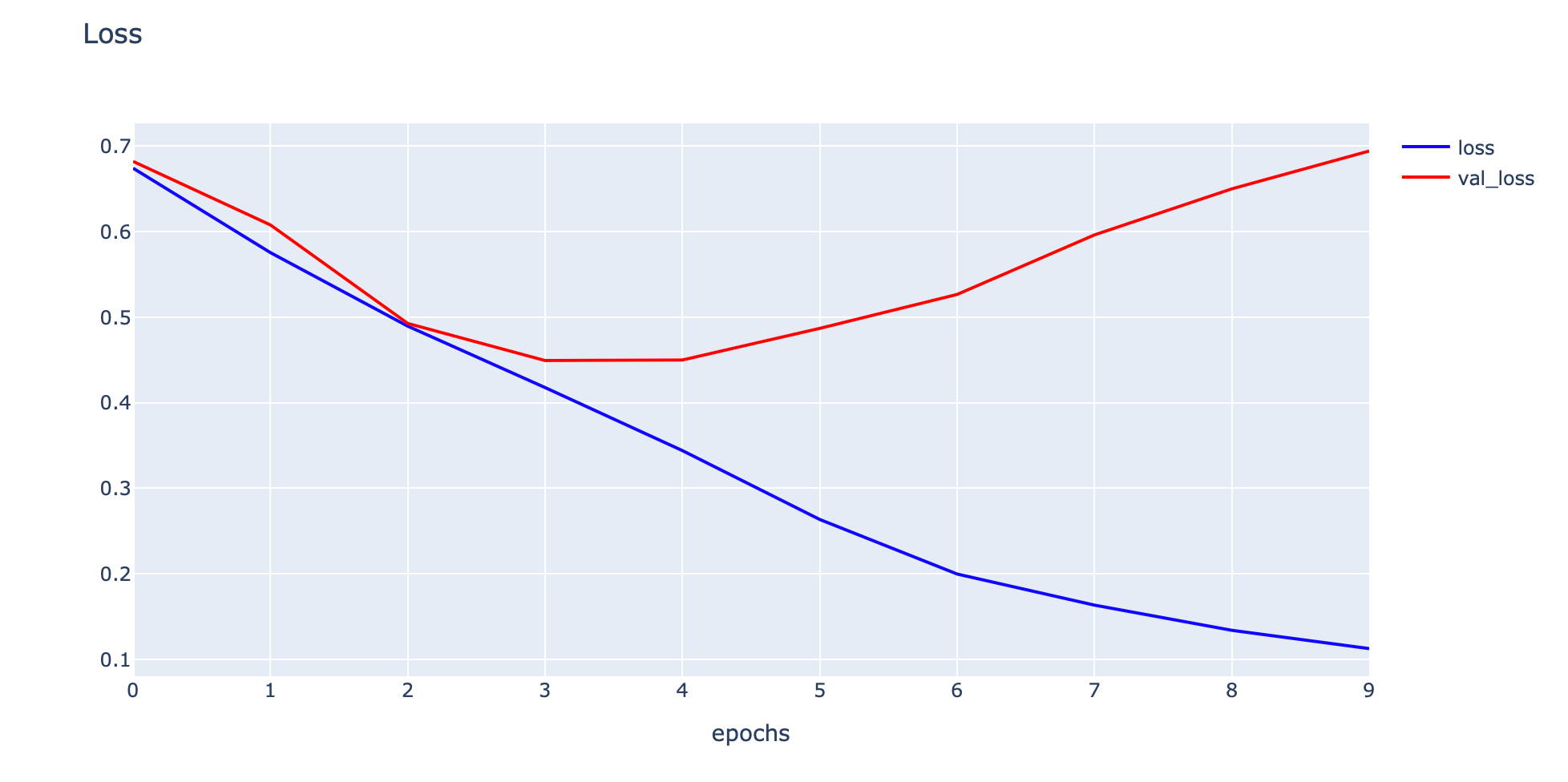

• Plot Accuracy และ Validate Accuracy

h1 = go.Scatter(y=his['accuracy'], 
                    mode="lines", line=dict(
                    width=2,
                    color='blue'),
                    name="acc"
                   )
h2 = go.Scatter(y=his['val_accuracy'], 
                    mode="lines", line=dict(
                    width=2,
                    color='red'),
                    name="val_acc"
                   )

data = [h1,h2]
layout1 = go.Layout(title='Accuracy',
                   xaxis=dict(title='epochs'),
                   yaxis=dict(title=''))
fig1 = go.Figure(data = data, layout=layout1)
fig1.show()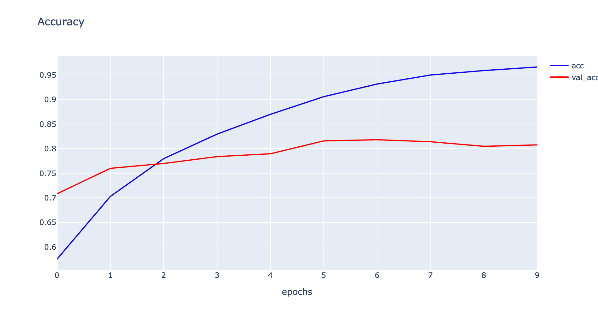

• Load และ Print ชนิดของ Layer, Output Shape และจำนวน Parameter ของ Model

predict_model = load_model(filename) 
predict_model.summary()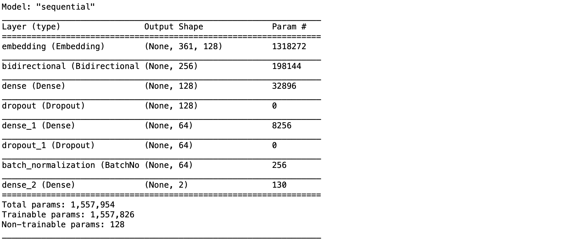

• Evaluate Model

score = predict_model.evaluate(val_X, val_Y, verbose=0)
print('Validate loss:', score[0])
print('Validate accuracy:', score[1])

• Predict ด้วย Validate Dataset

predicted_classes = np.argmax(predict_model.predict(val_X), axis=-1)
predicted_classes.shape

• เปลี่ยน y_true จาก One Hot กลับเป็นเลขจำนวนเต็มฐานสิบ

y_true = np.argmax(val_Y,axis = 1)
print(val_Y[0])
print(y_true[0])

• Save Confusion Matrix

cm = confusion_matrix(y_true, predicted_classes)
np.savetxt("confusion_matrix.csv", cm, delimiter=",")

• Plot Confusion Matrix

import seaborn as sn
import matplotlib.pyplot as plt

df_cm = pd.DataFrame(cm, range(2), range(2))
plt.figure(figsize=(20,14))
sn.set(font_scale=1.2) # for label size
sn.heatmap(df_cm, annot=True, annot_kws={"size": 14}, fmt='g') # for num predict size

plt.show()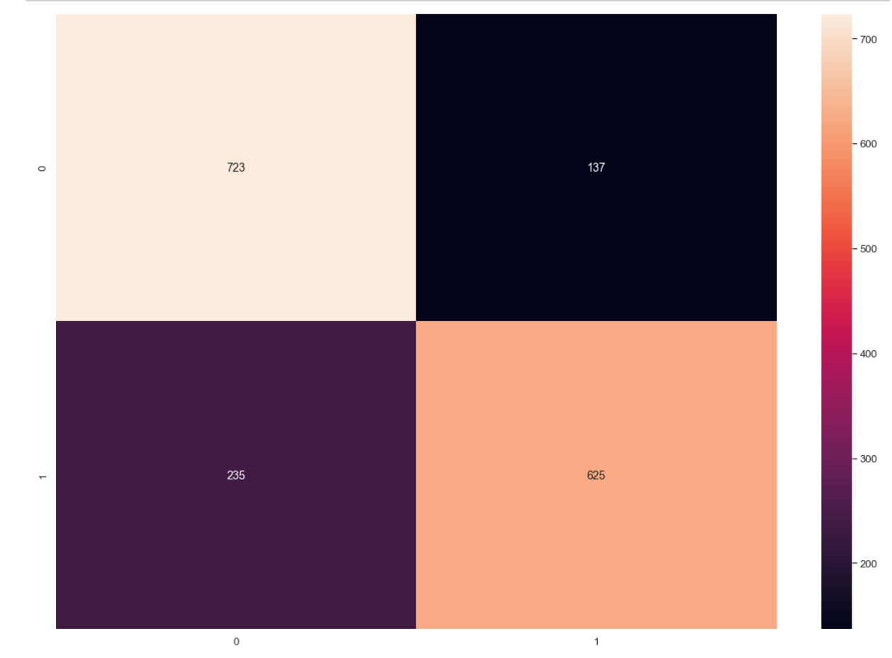

• ดึง Intent ทั้งหมดมาจาก output_tokenizer

label_dict = output_tokenizer.word_index

• ดึงชื่อของ Intent เก็บใน Label

label = [key for key, value in label_dict.items()]

• แสดง Precision, Recall, F1-score

print(classification_report(y_true, predicted_classes, target_names=label, digits=4))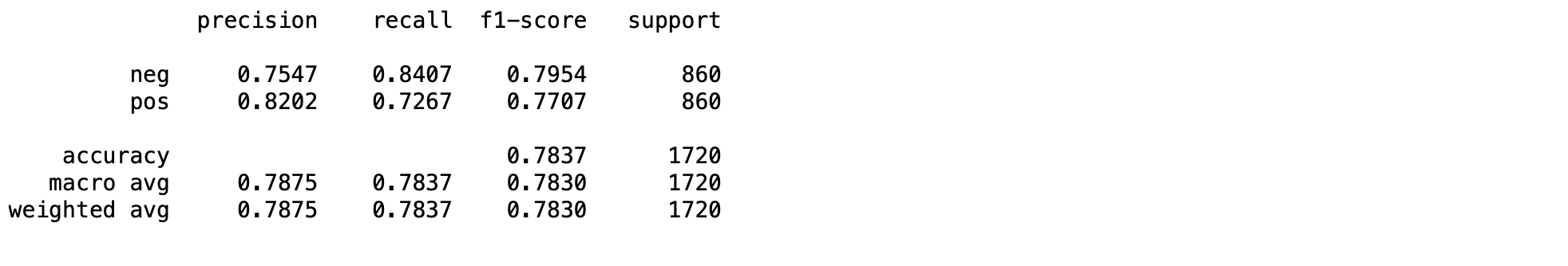

ทดลองเปลี่ยน Model แบบ GRU เป็น LSTM

• เราสามารถเปลี่ยนไปใช้ Model แบบ LSTM ได้ โดยปรับเปลี่ยนที่การนิยาม Model โดยเปลี่ยนจาก Bidirectional(GRU(128, activation = "relu")) เป็น Bidirectional(LSTM(128),merge_mode="concat")

model.add(Bidirectional(LSTM(128),merge_mode="concat"))

  สำหรับ  parameter ที่ชื่อว่า merge_mode ของ LSTM นั้นหมายถึง วิธีการนำ Vector มาต่อกัน ซึ่งนอกจากต่อแบบ concat แล้ว ยังมีการต่อแบบอื่น ๆ คือ sum, mul และ ave

• ขอบคุณ Wisesight (Thailand) Co., Ltd. สำหรับ Dataset

โบนัส สร้าง Word2Vec โดยใช้ Gensim คลิ๊กที่นี่ > Word2Vec Transfer Learning