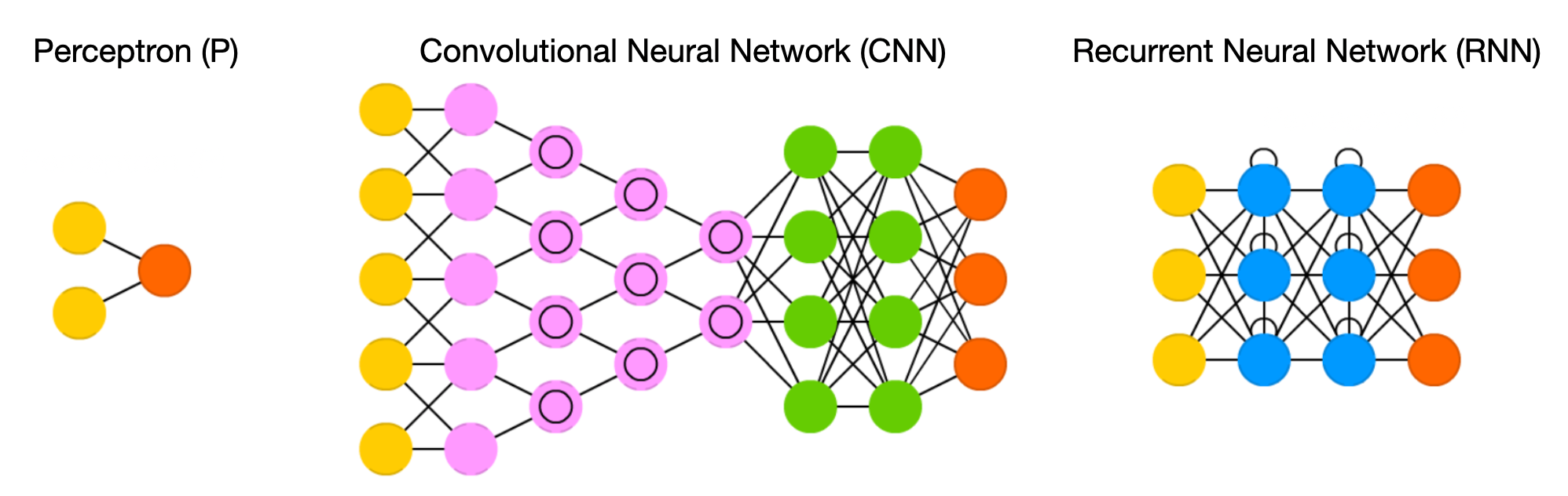
Implement the Back-propagation Algorithm from Scratch with NumPy

บทความโดย ผศ.ดร.ณัฐโชติ พรหมฤทธิ์
ภาควิชาคอมพิวเตอร์
คณะวิทยาศาสตร์
มหาวิทยาลัยศิลปากร

บทความโดย อ.ดร.ณัฐโชติ พรหมฤทธิ์ในบทความนี้เราจะศึกษา Neural Network อย่างละเอียดขึ้น ด้วยการทำความเข้าใจ Back-propagation Algorithm ซึ่งเป็นกระบวนการที่สำคัญในการย้อนกลับ (Backward) เพื่อปรับ Parameters (Weight และ Bias) ของ Model  เพื่อให้เข้าใจได้ง่ายที่สุด ผู้เขียนจึงได้ลดความซับซ้อนของ Model โดยใช้ Perceptron Neural Network เป็นตัวอย่างประกอบการอธิบาย แล้วทดลอง Implement Neural Network ที่มีความซับซ้อนเพิ่มขึ้นด้วย NumPy Library ครับ

Perceptron

Perceptron (P) เป็น Neural Network อย่างง่าย ที่จำลองการทำงานของเซลล์ประสาทมนุษย์ โดยจากภาพด้านบนซ้ายมือ เราเรียก Input Node ที่มี Cell ประสาท จำนวน 2 Cell ว่า Input Layer และ Output Node ที่มี Cell ประสาท จำนวน 1 Cell ว่า Output Layer แต่เนื่องจาก Input Layer ของ Neural Network ก็คือ Input Data ที่เป็นข้อมูลแบบ Scalar, Vector หรือ Matrix ไม่ใช่ Function เหมือนกับ Node ต่างๆ ใน Layer อื่น ตามธรรมเนียมมันจึงไม่ถูกนับเป็น 1 Layer ด้วย ดังนั้น Perceptron จึงมี Layer ทั้งหมด 1 Layer ครับ

Forward Propagation

Input Layer

จากภาพด้านบน Node ที่มีสีฟ้า คือ Input Data (Xi) ที่จะเป็นข้อมูลแบบ Scalar, Vector หรือ Matrix

Xi, i ∈ 1, 2

Output Layer

ส่วน Layer สุดท้ายของ Neural Network คือ Output Layer ที่เป็น Node สีส้ม และ Node สีนำ้ตาล โดยที่ Node สีส้ม จะมีการนำ Weight ที่เกิดจากการสุ่มในช่วงเริ่มต้นของการ Train คูณกับ Input Data แล้วนำผลลัพธ์จากการคูณมาบวกกับ Bias (B) ซึ่งเกิดจากการสุ่มในช่วงเริ่มต้นเช่นกัน

Z = W · X + B

ในการ Implement เราจะแทน Weight (W) ด้วย Matrix ขนาด mxn โดย m คือจำนวน Output Node (ในที่นี้มี 1 Node) และ n คือ จำนวน Input Node (ในที่นี้มี 2 Node)

W = [w1 w2] 

ขณะที่ X จะเป็น Matrix ขนาด nx1 ที่แทนกลุ่มของ Input Node

และ B เป็น Matrix ขนาด mx1

B = [b]

ดังนั้นเราคำนวณ Z ได้ดังนี้

สมมติว่า X, W และ B เป็น Neural Network ดังในภาพด้านล่าง และ Z = [z] ดังนั้น Z จะเท่ากับ 0.36

Z = [w1x1 + w2x2] + [b]
  = [(0.2)(0.05) + (0.5)(0.1)] + [0.3]
  = [0.36] 

Activate Function

แต่ก่อนที่จะส่งผลลัพธ์ออกมา เราจะนำมันมาปรับค่าด้วย Activate Function เพื่อทำให้มันอยู่ในช่วง 0 - 1 ซึ่งเราเรียกฟังก์ชันสำหรับการปรับค่าอย่างนี้ว่า Sigmoid Function

sigmoid(z) = 1/(1+e^(-z))

ดังนั้นผลลัพธ์สุดท้ายที่เป็นค่าที่ Model ทำนายออกมาได้ หรือ ŷ จะเท่ากับ Sigmoid(z)

ŷ = Sigmoid(z) = Sigmoid(0.36) = 0.5890

Loss Function

ขั้นตอนสุดท้ายของการทำ Forward Propagation คือการประเมินว่าผลการ Predict คลาดเคลื่อนจาก Output y มากน้อยเพียงใด ด้วย Loss Function (L) =  Loss(y, ŷ) โดยที่ L อาจจะเป็น MSE (Mean Squared Error) หรือ Cross-entropy ฯลฯ

สมมติว่า y เท่ากับ 0.7 และ L คือ MSE ดังนั้น L จะมีค่าเท่ากับ 0.0123

L = Loss(y,ŷ) 
  = (y - ŷ)^2 
  = (0.7 - 0.589)^2 = 0.0123

Back-propagation

เราสามารถทำกระบวนการ Backward Propagation เพื่อปรับค่า w1 จากการหาอนุพันธ์ของ L เทียบกับ w1 หรือความชัน (Gradient) ของ Loss(y, ŷ) หรือ Error ที่ w1 ด้วยสมการด้านล่าง

แต่เนื่องจากไม่มี w1 ใน L เราจึงต้องใช้กฎลูกโซ่ (Chain Rule)

หาค่าในแต่ละ Term

ดังนั้น Error_at_w1 = (-0.222)(0.242)(0.05) = -0.003

กำหนดให้ Learning Rate เท่ากับ 0.5 ปรับค่า w1 ได้ดังนี้

Update w1 = w1 - Learning_Rate*Error_at_w1
          = 0.2-(0.5)(-0.003)
          = 0.2015

Implement with NumPy

เราจะทดลอง Implement Neural Network โดยเพิ่มความซับซ้อนของ Model อีกเล็กน้อย ดังภาพด้านล่าง

นิยาม Neural Network Model

นิยาม Neural Network Model ที่ไม่ใส่ Bias

import numpy as np
import pandas as pd
from matplotlib import pyplot as plt  
from sklearn.datasets import make_blobs
import plotly
import plotly.graph_objs as go
def create_nn_model(x, y, l):
    input_layer = x
    weights1 = np.random.uniform(-1, 1, (input_layer.shape[1], 4))
    
    weights2 = np.random.uniform(-1, 1, (4, 1))
    label = y
    output_layer = np.zeros(y.shape)
    learning_rate = l
    
    return {'input_layer': input_layer, 'weights1': weights1, 'weights2': weights2, 'label': label, 'output_layer': output_layer, 'learning_rate': learning_rate}

สร้าง Dataset ที่มี Input Feature เท่ากับ 3 (มิติ) และผลเฉลยเป็น 0 และ 1 จำนวน 10 Record ด้วยฟังก์ชัน make_blobs

x, y = make_blobs(n_samples=10, centers=2, n_features=3)

y = np.expand_dims(y, axis=1)
x.shape, y.shape

((10, 3), (10, 1))

สร้าง กำหนด Learning Rate แล้วสร้าง Model

learning_rate = 0.1

model = create_nn_model(x, y, learning_rate)

แสดง Shape ของ Input Layer

model['input_layer'].shape

(10, 3)

แสดง Data ที่อยู่ใน Input Layer

model['input_layer']

แสดง Shape ของ Weight1

model['weights1'].shape

(3, 4)

แสดงค่าเริ่มต้นของ Weight1

model['weights1']

แสดง Shape ของ Weight2

model['weights2'].shape

(4, 1)

แสดงค่าเริ่มต้นของ Weight2

model['weights2']

แสดง Shape ของผลเฉลย

model['label'].shape

(10, 1)

แสดงค่าของผลเฉลย

แสดง Shape ของ Output Layer

model['output_layer'].shape

(10, 1)

แสดงค่าเริ่มต้นของ Output Layer

model['output_layer'] #ŷ

นิยาม Sigmoid Activate Function และอนุพันธ์ของ Sigmoid

def sigmoid(x):
    return 1.0/(1+ np.exp(-x))

def sigmoid_derivative(x):
    return x * (1.0 - x)

นิยาม Loss Function (L)

def loss(model):
    return sum((model['label'] - model['output_layer'])**2)

นิยาม Feed Forward Function

def feedforward(model):
    model['layer1'] = sigmoid(np.dot(model['input_layer'], model['weights1']))
    model['output_layer'] = sigmoid(np.dot(model['layer1'], model['weights2']))               

นิยาม Back-propagation Function เพื่อปรับค่า weights2 และ weights1

def backprop(model):
    d_weights2 = np.dot(model['layer1'].T, (2*(model['label']- model['output_layer']) * sigmoid_derivative(model['output_layer'])))
    d_weights1 = np.dot(model['input_layer'].T,  (np.dot(2*(model['label'] - model['output_layer']) * sigmoid_derivative(model['output_layer']), model['weights2'].T) * sigmoid_derivative(model['layer1'])))
    
    model['weights2'] += model['learning_rate']*d_weights2
    model['weights1'] += model['learning_rate']*d_weights1

Train Model

history=[]
epoch = 500

for i in range(epoch):
    feedforward(model)
    backprop(model)
    history.append(loss(model))

Plot Loss

df = pd.DataFrame(history, columns=['loss'])
df.head()
h1 = go.Scatter(y=df['loss'], 
                    mode="lines", line=dict(
                    width=2,
                    color='blue'),
                    name="loss")

data = [h1]

layout1 = go.Layout(title='Loss',
                   xaxis=dict(title='Epochs'),
                   yaxis=dict(title=''))
fig1 = go.Figure(data, layout=layout1)
plotly.offline.iplot(fig1)

ลองทำดู

  • ปรับ Learning Rate ตั้งแต่ 0.1, 0.2, ..., 1.0 แต่ละค่า Train 1,000 Epoch
  • Plot Loss จากการปรับ learning_rate 10 ค่า รวมกัน
  • วิเคราะห์ผลการทดลอง